Top Valorant Players

Author: Ethan Tran (ethankt1@uci.edu)
Course Project
UC Irvine
Math 10 | Spring 2024
I would like to post my notebook on the course’s website. [Yes]

Introduction

This is a dataset of the highest-ranking players from Riot Games’, Valorant. The game features a 5v5 objective-based matches where the mechanics include an economy system for purchasing various weapons (emphasizing precise gameplay) and strategic planning. The goal of this analysis is to show if there are any relationships in the data visually amongst the top players in the world.

Import libraries

import numpy as np
import pandas as pd 
import matplotlib.pyplot as plt
import seaborn as sns
from sklearn.linear_model import LinearRegression, LogisticRegression, ElasticNet
from sklearn.model_selection import train_test_split
from sklearn.metrics import accuracy_score, mean_squared_error, r2_score
from sklearn.preprocessing import StandardScaler
from sklearn.ensemble import RandomForestRegressor

Load Data

df = pd.read_csv("val_stats.csv")
df

/var/folders/_h/2nwpq18d7c13g7t5z53xhw6r0000gn/T/ipykernel_77938/3110898118.py:1: DtypeWarning: Columns (0,10) have mixed types. Specify dtype option on import or set low_memory=False.
  df = pd.read_csv("val_stats.csv")

	region	name	tag	rating	damage_round	headshots	headshot_percent	aces	clutches	flawless	...	gun2_name	gun2_head	gun2_body	gun2_legs	gun2_kills	gun3_name	gun3_head	gun3_body	gun3_legs	gun3_kills
0	NaN	ShimmyXD	#NA1	Radiant	135.8	992	24.9	0	140	80	...	Phantom	33	62	5	220	Classic	36	60	3	147
1	NaN	XSET Cryo	#cells	Radiant	170.3	879	28.3	2	122	94	...	Operator	8	91	0	226	Phantom	32	63	5	137
2	NaN	PuRelittleone	#yoruW	Radiant	147.5	720	24.0	3	117	59	...	Phantom	36	61	3	231	Operator	8	91	1	102
3	NaN	Boba	#0068	Radiant	178.2	856	37.3	3	83	49	...	Sheriff	48	51	1	48	Phantom	44	56	0	36
4	NaN	i love mina	#kelly	Radiant	149.8	534	24.4	2	71	38	...	Spectre	21	71	8	65	Operator	8	92	0	64
...	...	...	...	...	...	...	...	...	...	...	...	...	...	...	...	...	...	...	...	...	...
85673	LAT	Kazutora	#img0d	Radiant	138.2	342	21.4	0	58	54	...	Vandal	28	69	2	175	Classic	39	59	2	71
85674	LAT	el lobo marino	#uthur	Radiant	182.9	650	30.1	4	77	42	...	Vandal	40	57	3	212	Spectre	33	63	5	139
85675	LAT	p9pzet	#666x	Radiant	158.8	613	30.2	0	70	54	...	Phantom	40	56	4	159	Operator	10	89	1	87
85676	LAT	EZ4TGD EnSBuwu	#kmeve	Immortal 3	155.9	132	22.2	0	23	18	...	Phantom	39	57	3	37	Spectre	27	69	4	17
85677	LAT	Neon	#SSJ	Radiant	164.4	1,127	20.7	3	136	82	...	Operator	9	88	2	132	Spectre	27	70	2	108

85678 rows × 38 columns

df.columns

Index(['region', 'name', 'tag', 'rating', 'damage_round', 'headshots',
       'headshot_percent', 'aces', 'clutches', 'flawless', 'first_bloods',
       'kills', 'deaths', 'assists', 'kd_ratio', 'kills_round', 'most_kills',
       'score_round', 'wins', 'win_percent', 'agent_1', 'agent_2', 'agent_3',
       'gun1_name', 'gun1_head', 'gun1_body', 'gun1_legs', 'gun1_kills',
       'gun2_name', 'gun2_head', 'gun2_body', 'gun2_legs', 'gun2_kills',
       'gun3_name', 'gun3_head', 'gun3_body', 'gun3_legs', 'gun3_kills'],
      dtype='object')

Copy Data (Numeric-only)

Using numerical data is often better for analysis because it is more computationally efficient, reduces noise, and leads to more accurate and reliable insights.

numeric_df = df.select_dtypes(include=['int64', 'float64'])
numeric_df.to_csv("val_stats_numeric.csv", index=False)

Visualize Data

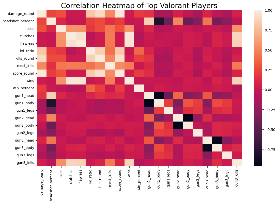
Correlation Heatmap

fig, ax = plt.subplots(figsize=(13, 8))
sns.heatmap(numeric_df.corr())
plt.title('Correlation Heatmap of Top Valorant Players', fontsize=20)
plt.show()

Context:

In Valorant, a players’ weapon choice significantly impacts gameplay. Among the 17 different weapons, the top-three weapons, “Gun[1-3]”, stand out as the most frequently used by players. (Gun 1 being the most-favored weapon of choice, Gun 3 being the 3rd most-favored)

for i in range(1,4):
    colors = ["red","blue","green"]
    fig, ax = plt.subplots(figsize = (15,5))
    
    plt.hist(df["gun{}_name".format(i)], bins = 64, edgecolor="Black", facecolor = colors[i-1])
    plt.title("Gun {} and number of eliminations".format(i).title(),fontsize = 20)
    plt.xlabel("Gun name:",fontsize = 15)
    plt.ylabel("Number of eliminations",fontsize = 15)
    plt.show()

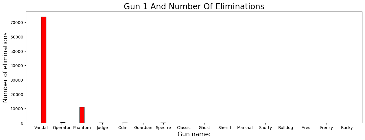
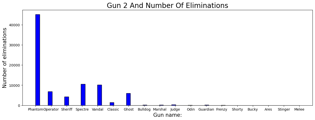
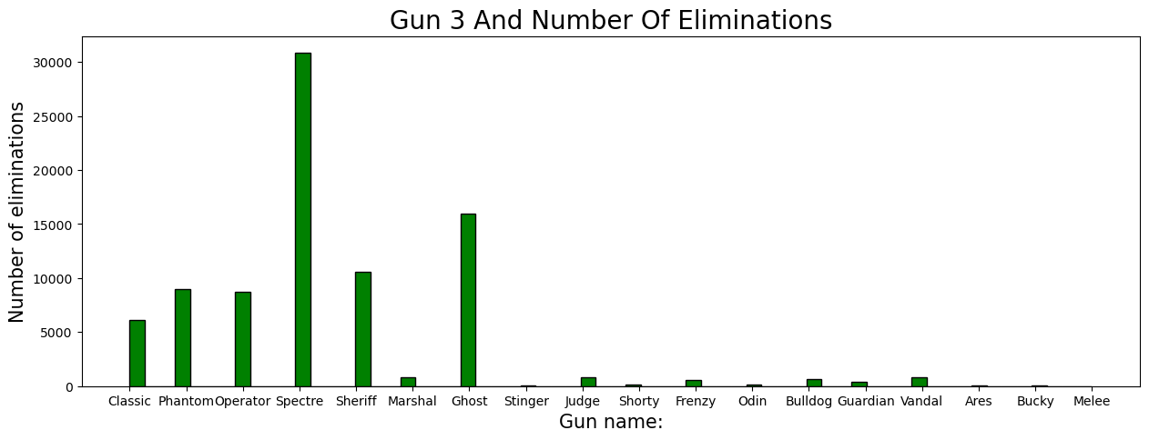
Shown by the histogram, the most preferred weapon is the “Vandal”. Second most preferred is the “Phantom”. Lastly, “Spectre” as the third.

Linear Regression

X = df[['damage_round']]
y = df['kd_ratio']

model = LinearRegression()
model.fit(X, y)
lm = model.predict(X)

print(f"Coefficient: {model.coef_[0]}")
print(f"Intercept: {model.intercept_}")
print(f"R-squared: {model.score(X, y)}")

plt.figure(figsize=(10, 7))
sns.scatterplot(x='damage_round', y='kd_ratio', data=numeric_df, alpha=0.5, label='Actual data')
plt.plot(df['damage_round'], lm, color='red', label='Regression line')
plt.xlabel('Damage per Round')
plt.ylabel('K/D Ratio')
plt.title('Linear Regression: Damage per Round vs. K/D Ratio')
plt.legend()
plt.show()

Coefficient: 0.0077748624852823425
Intercept: -0.05643181253842333
R-squared: 0.6629070657865264

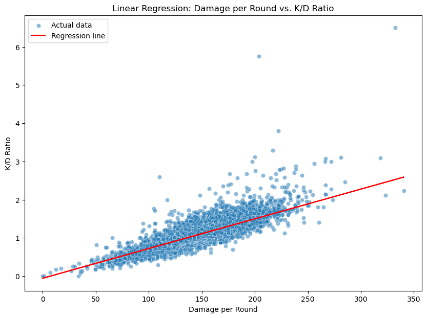
As shown through the linear regression model, these players’ ability to consistently deal significant damage while maintaining a high kill/death ratio is indicative of their overall impact and importance within competitive play. Since kills and damage are highly correlated, it was inevitable that this was going to be a positive trend; however, when taking into account the amount of deaths, it is more interesting to see if there were any outliers among the top players.

Logistic Regression

We will use logistic regression to predict whether a player is a “duelist” based on the average number of kills per round. Duelists are agents known to engage in direct combat and secure kills. Stereotypically, these are supposed to be the ones with the highest amount of kills.

duelist_agents = ['Jett', 'Phoenix', 'Raze', 'Reyna', 'Yoru', 'Neon']
df['isDuelist'] = df['agent_1'].isin(duelist_agents).astype(int)

Train Test Split & Accuracy

X = df[['kills_round']]
y = df['isDuelist']      

X_train, X_test, y_train, y_test = train_test_split(X, y, test_size=0.5, random_state=1)
model = LogisticRegression()
model.fit(X_train, y_train)
y_pred = model.predict(X_test)

accuracy = accuracy_score(y_test, y_pred)
print("Accuracy of logistic regression model:", accuracy)

Accuracy of logistic regression model: 0.6604729335418661

An accuracy score of 66% indicates that the model’s ability to correctly classify agents as duelists or non-duelists based on average kills per round is slightly above average.

Sigmoid Function

By mapping the output to a probability value between 0 and 1, the sigmoid function makes it possible to interpret the results of logistic regression. This graph should make it easier to predict the probability of being a duelists based on KPR

X_range = np.linspace(X['kills_round'].min(), X['kills_round'].max(), 300)
z = model.coef_ * X_range.reshape(-1,1) + model.intercept_ 
y_prob = 1 / (1 + np.exp(-z))

plt.figure(figsize=(10, 6))
sns.scatterplot(x='kills_round', y='isDuelist', data=df, alpha=0.5, label='Actual data')
plt.plot(X_range, y_prob, color='red', label='Logistic regression curve (Sigmoid)')
plt.xlabel('Kills per Round (KPR)')
plt.ylabel('Probability of Being a Duelist')
plt.title('Logistic Regression: Probability of Being a Duelist vs. Kills per Round')
plt.legend()
plt.show()

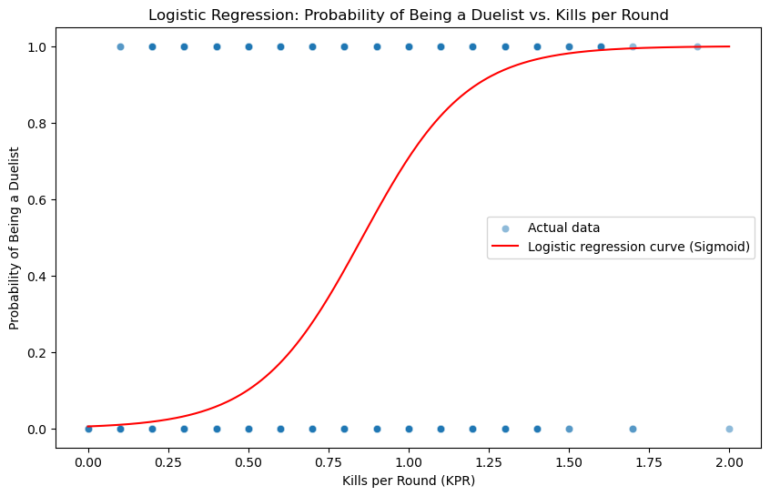
This logistic regression shows that having a high kill per round (KPR) does not necessarily mean that you are a duelist. While duelists are often associated with high kill counts, other roles also contribute significantly to team success through non-kill-related actions. However, in higher-ranked matches, we can see that it may be impossible to predict whether or not someone is playing a “duelist” solely based off KPR. Unfortunately, KPR is calculated to the nearest tenth so we will not get accurate depictions of where exactly is the mean KPR. On the other hand, it does not matter in this case since predicting the role of the character does not cause higher/lower KPR.

Box Plot

Since KPR and the probability of being a duelist is not interesting enough, how about seeing it through the lens of all agents?

plt.figure(figsize=(14, 8))
sns.boxplot(x='kills_round', y='agent_1', data=df)
plt.xlabel('Kills per Round')
plt.ylabel('Agent')
plt.title('Box Plot of Kills per Round by Agent')
plt.show()

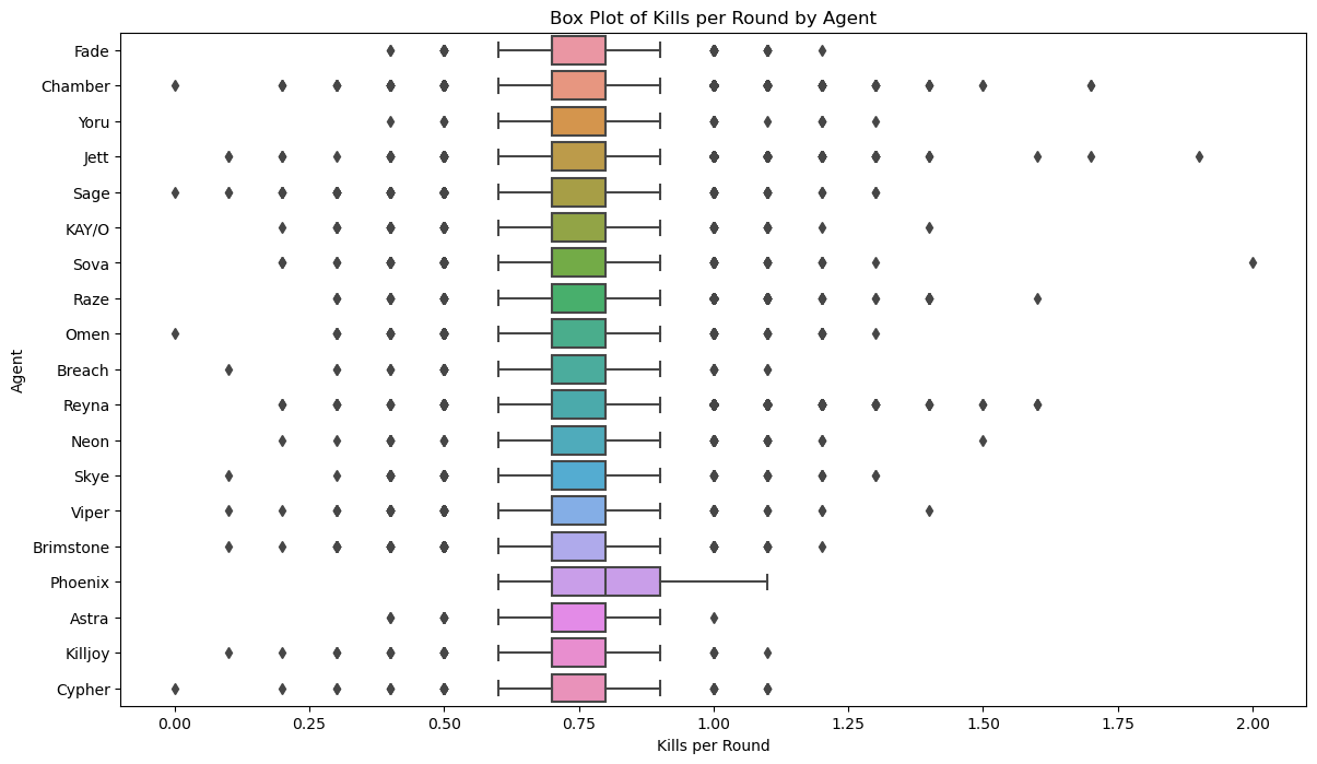
Here we can see that the median of every agent is around 0.75 KPR, but what is interesting is the amount of disparity/outliers coming from each agent. Based on the many box plots, we can clearly see that our hypothesis was correct about agents not having the biggest effect on kills.

ElasticNet

ElasticNet is a linear model that combines the properties of both Lasso (L1) and Ridge (L2) regression.

X = df[['kills_round', 'damage_round', 'headshot_percent', 'score_round']]
y = df['win_percent']
X_train, X_test, y_train, y_test = train_test_split(X, y, test_size=0.5, random_state=1)

Selecting these features might be irrelevant to the modeling process. However, since KPR and Score per Round (SPR) are highly correlated along with damage and headshot percentage, it might be useful since it can handle multicollinearity.

Feature Scaling

scaler = StandardScaler()
X_train_scaled = scaler.fit_transform(X_train)
X_test_scaled = scaler.transform(X_test)

With the combined property of both Lasso and Ridge regression, its important to address the regularization that comes with it. By scaling, it lets all features contribute equally so that one does not effect the other drastically.

elastic_net = ElasticNet(alpha=0.1, l1_ratio=0.5)
elastic_net.fit(X_train_scaled, y_train)
y_pred = elastic_net.predict(X_test_scaled)

r2 = r2_score(y_test, y_pred)
mse = mean_squared_error(y_test, y_pred)
print("ElasticNet Coefficients:", elastic_net.coef_)
print("ElasticNet Intercept:", elastic_net.intercept_)
print("ElasticNet R-squared:", r2)
print("ElasticNet Mean Squared Error:", mse)

ElasticNet Coefficients: [ 2.18967798  0.33484552 -0.53189074  0.        ]
ElasticNet Intercept: 53.83205957188543
ElasticNet R-squared: 0.04880163146877592
ElasticNet Mean Squared Error: 125.29573107476482

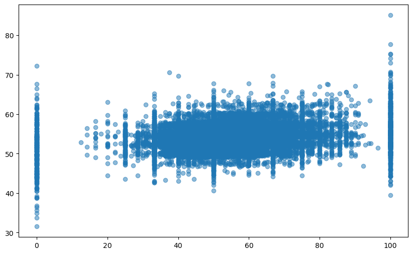
With such a high MSE, it might be that the model has made an error in predicting the target variable. However, this would be the case since there are so many different factors to predicting win percentage. In a matchmaking system of 5v5 of the top players, even having one player not having the best day could throw this graph off and cause their own team to lose.

plt.figure(figsize=(10, 6))
plt.scatter(y_test, y_pred, alpha=0.5)
plt.plot([y_test.min(), y_test.max()], [intercept + coefficients * y_test.min(), intercept + coefficients * y_test.max()],
         color='red', label='Regression Line')
plt.xlabel('Actual Win Percentage')
plt.ylabel('Predicted Win Percentage')
plt.title('ElasticNet Regression: Actual vs Predicted Win Percentage')
plt.show()

---------------------------------------------------------------------------
NameError                                 Traceback (most recent call last)
Cell In[34], line 3
      1 plt.figure(figsize=(10, 6))
      2 plt.scatter(y_test, y_pred, alpha=0.5)
----> 3 plt.plot([y_test.min(), y_test.max()], [intercept + coefficients * y_test.min(), intercept + coefficients * y_test.max()],
      4          color='red', label='Regression Line')
      5 plt.xlabel('Actual Win Percentage')
      6 plt.ylabel('Predicted Win Percentage')

NameError: name 'intercept' is not defined

Random Forest Regressor

Unlike ElasticNet producing coefficients, Random Forest fits a number of decision tree regressors on a number of samples that are averaged in order to improve the accuracy in predictions.

rf = RandomForestRegressor(n_estimators=10, random_state=1)
rf.fit(X_train_scaled, y_train)
y_pred_rf = rf.predict(X_test_scaled)

r2_rf = r2_score(y_test, y_pred_rf)
mse_rf = mean_squared_error(y_test, y_pred_rf)
print("Random Forest R-squared:", r2_rf)
print("Random Forest Mean Squared Error:", mse_rf)

plt.figure(figsize=(10, 6))
plt.scatter(y_test, y_pred_rf, color='green', alpha=0.5)
plt.xlabel('Actual Win Percentage')
plt.ylabel('Predicted Win Percentage')
plt.title('Random Forest Regression: Actual vs Predicted Win Percentage')
plt.show()

Overall, since there are not enough features, the regression techniques are not enough to accurately depict actual vs predicted win percentages. In this case, regularization should not be used since it discourages a more complex model in preventing overfitting.

Summary

Overall, the analysis provides valuable insight into the Top Valorant Players dataset, helping to understand player behavior, performance factors, and the extremities of stereotypes. This analysis can inform strategies for improving player mindset while optimizing gameplay tactics in Valorant. What should be kept into mind is that win percentage in Valorant is shaped not only by individual gameplay statistics, but also by effective communication, teamwork tactics, etc.

References

• https://www.kaggle.com/datasets/aliibrahim10/valorant-stats/data

• https://rayzhangzirui.github.io/math10sp24/notes/pandas.html

• https://rayzhangzirui.github.io/math10sp24/notes/visualization.html

• https://rayzhangzirui.github.io/math10sp24/notes/logistic_binary.html

• https://elitedatascience.com/algorithm-selection

• https://scikit-learn.org/stable/modules/generated/sklearn.ensemble.RandomForestRegressor.html