Probability and Statistics#
These concepts are foundational in data science, enabling us to quantify uncertainty and variability in data.
Random Variables#
Discrete Random Variables#
Consider a random experiment where we roll a fair six-sided die. The result is uncertain, embodying a discrete random variable, which we can denote as \(X\). This variable \(X\) can take one of a finite set of values, each with its own probability.
Example: If \(X\) represents the outcome of rolling a die, then \(X \in \{1, 2, 3, 4, 5, 6\}\), with \(P(X = x) = \frac{1}{6}\) for each \(x \in \{1, 2, 3, 4, 5, 6\}\).
Continuous Random Variables#
In contrast, consider measuring the time it takes for the next bus to arrive, which might be any positive real number. Here, we have a continuous random variable, say \(Y\), which can take any value within an interval.
Example: If \(Y\) denotes the time (in minutes) for the next bus to arrive, then \(Y \in [0, \infty)\). Here, \(Y\) could be 2.5 minutes, 3.14159 minutes, or any other positive real number.
Distributions#
The probability distribution of a random variable provides a complete description of the likelihood of various outcomes.
For a discrete variable \(X\), the probability mass function (PMF) gives \(P(X = x)\) for each possible \(x\).
For a continuous variable \(Y\), the probability density function (PDF), \(f_Y(y)\), is such that the probability of \(Y\) falling in an interval \([a, b]\) is given by \(\int_a^b f_Y(y) \, dy\).
Expectation#
The expectation or expected value of a random variable provides a measure of the central tendency of its distribution.
For a discrete random variable \(X\), \(E[X] = \sum_{x} x \cdot P(X = x)\).
For a continuous random variable \(Y\), \(E[Y] = \int_{-\infty}^{\infty} y \cdot f_Y(y) \, dy\).
You can always think of the random variable as the “payoff” in a game, and the expectation is the “average payoff” in each round of the game if you play it many times.
We have \(E[aX + bY] = aE[X] + bE[Y]\) for any constants \(a\) and \(b\).
How to estimate the expectation of a random variable from data?#
One common approach is to use the sample mean: if \(X_1, X_2, \ldots, X_n\) are independent and identically distributed (i.i.d.) samples of \(X\), then the sample mean \(\bar{X} = \frac{1}{n} \sum_{i=1}^{n} X_i\) is an estimator of \(E[X]\)
Variance#
Variance quantifies the spread of a distribution around its mean, reflecting the variability of the random variable. \(\text{Var}(X) = E[(X - E[X])^2]\)
Alternatively, we can compute the variance as \(\text{Var}(X) = E[X^2] - (E[X])^2\): \begin{align*} \text{Var}(X) & = E[(X - E[X])^2] \ & = E[X^2 - 2XE[X] + (E[X])^2] \ & = E[X^2] - 2E[X]E[X] + (E[X])^2 \ & = E[X^2] - (E[X])^2. \end{align*} The key here is that E[X] is a constant: it’s an property of the distribution of X, not a random variable.
How to estimate the variance of a random variable from data?#
One common approach is to use the sample variance: if \(X_1, X_2, \ldots, X_n\) are i.i.d. samples of \(X\), then the sample variance \(S^2 = \frac{1}{n} \sum_{i=1}^{n} (X_i - \bar{X})^2\) is an estimator of \(\text{Var}(X)\). (This is not an “unbiased estimator” in statistics, no need to worry about that in this course)
Standard Deviation#
The standard deviation is the square root of the variance, \(\sigma^2 = \text{Var}(X)\), providing a measure of the spread of a distribution in the same units as the random variable.
Covariance#
Covariance provides a measure of how two random variables change together. For example, if we treat weight and height as random variables, then knowing that someone is taller than average might make it more likely that they have above-average weight.
For random variables \(X\) and \(Y\), the covariance is defined as \(\text{Cov}(X, Y) = E[(X - E[X])(Y - E[Y])]\).
Using the linearity of expectation, we also have \(\text{Cov}(X, Y) = E[XY] - E[X] \cdot E[Y]\).
Correlation#
Correlation is a standardized measure of how two random variables change together, ranging from -1 to 1. \( \text{Corr}(X, Y) = \frac{\text{Cov}(X, Y)}{\sqrt{\text{Var}(X) \cdot \text{Var}(Y)}}\).
Independence#
Intuitively, when two things are independent, the outcome of one does not influence the outcome of the other.
Two random variables, \(X\) and \(Y\), are considered independent if \(P(X = x, Y = y) = P(X = x) P(Y = y)\) for all \(x\) and \(y\). Intuitively, this means that knowing the value of one variable provides no information about the value of the other.
For example, if we flip two coins, and \(X\) and \(Y\) represent the outcomes of the first and second coin flips, respectively, then the outcomes are independent. The probability of getting two heads is \(P(X = \text{heads}) \cdot P(Y = \text{heads}) = \frac{1}{2} \cdot \frac{1}{2} = \frac{1}{4}\).
Independence and Covariance#
Independence implies zero covariance. But the converse is not necessarily true.
Exercise: If \(X\) and \(Y\) are independent, use the linearity of expectation to show that \(\text{Cov}(X, Y) = 0\).
Covariance and correlation only measure linear relationships between random variables. They can’t capture more complex relationships.
Example of zero covariance but not independence:
Consider a scenario where \(X\) is a random variable uniformly distributed over \([-1, 1]\) and define \(Y = X^2\). Now they are not independent: knowing \(X\) gives information about \(Y\).
Recall \(\text{Cov}(X, Y) = \mathbb{E}[X \cdot Y] - \mathbb{E}[X]\mathbb{E}[Y] = 0\). In this example, \(\mathbb{E}[X] = 0\), and \(XY = X^3\) is an odd function, so \(\mathbb{E}[X \cdot Y] = 0\) ( for every positive outcome, there is a corresponding negative outcome with the same probability).
Alternatively, recall the \(\text{Cov}(X, Y) = \mathbb{E}[(X - \mathbb{E}[X])(Y - \mathbb{E}[Y])] = 0\). \(E[X]\) is 0, and \(E[Y]\) is somewhere between 0 and 1. When \(X>E[X]\), \(Y\) could be smaller than or larger than \(E[Y]\). Therefore these two variable does not move in the same direction with respect to their means.
Causality#
Correlation is Not Causation#
Correlation measures the strength and direction of a linear relationship between two variables. However, it does not imply causation.
For example: Ice cream sales and drowning incidents might be correlated (both increase in the summer), but one does not cause the other.
See Spurious Correlations for more examples.
Independent is Not “No-Causation”#
Suppose two light switches, A and B, control the light bulb in the following way: the light is on if (1) A on B off or (2) A off B on. Assume the switch are independent “coin flips”: equally likely to be on or off. Then knowing the state of switch A gives no information about the light. But there is still a “cause and effect” relationship between the switch and the light. We only see this relationship when we consider both switches together. (Example adapted from here)
Establishing Causality#
Establishing causality is challenging, and might require controlled experiments beyond observational data.
Computation#
The following Python code demonstrates how to do computation related to the previous concepts.
Estimating probabilities#
When we don’t know the probability of some event, we can estimate it by running the experiment many times and calculating the relative frequency of the event.
# generate list of random integers
import numpy as np


# estimating the probability of rolling a 6
# n is number of experiments, or sample size
# larger n, "closer" to true probability
n = 100
x = np.random.randint(1, 7, n)
p = np.sum(x == 6) / 100
print(p)
0.19
# uniform distribution on [0, 1]
# estimating the probability hitting [0, 0.5]
n = 100
x = np.random.rand(n)
p = np.sum(x < 0.5) / n
print(p)
0.51
visualizing distribution using histogram#
# to install seaborn
# %conda install seaborn
# %pip install numpy
# %conda install numpy
# for to visualize the distribution, we can use a histogram
import matplotlib.pyplot as plt

n = 100
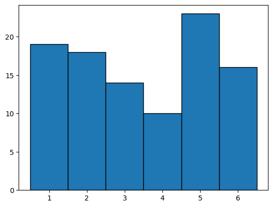
x = np.random.randint(1, 7, n)

plt.hist(x, bins=6, range=(0.5, 6.5),edgecolor='black')
(array([19., 18., 14., 10., 23., 16.]),
 array([0.5, 1.5, 2.5, 3.5, 4.5, 5.5, 6.5]),
 <BarContainer object of 6 artists>)
# can also use seaborn
# import seaborn
# seaborn.histplot(x, discrete=True)
# generate uniform random numbers
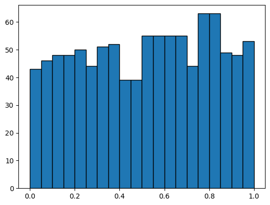
x = np.random.rand(1000)
# seaborn.histplot(x, stat='density')
plt.hist(x, bins=20, range=(0, 1), edgecolor='black')
(array([43., 46., 48., 48., 50., 44., 51., 52., 39., 39., 55., 55., 55.,
        55., 44., 63., 63., 49., 48., 53.]),
 array([0.  , 0.05, 0.1 , 0.15, 0.2 , 0.25, 0.3 , 0.35, 0.4 , 0.45, 0.5 ,
        0.55, 0.6 , 0.65, 0.7 , 0.75, 0.8 , 0.85, 0.9 , 0.95, 1.  ]),
 <BarContainer object of 20 artists>)
# gaussian normal distribution
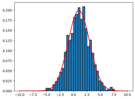
# as n increases, the histogram looks more like the density function
# mu is the mean, sigma is the standard deviation
mu = 1
sigma = 2
n = 1000 # sample size
x  = np.random.normal(mu, sigma, n) # generate samples from the normal distribution

# plot the histogram
plt.hist(x, bins=30, edgecolor='black', density=True)


# plot the density function
x = np.linspace(-10, 10, 100)
f = (1/(sigma * np.sqrt(2 * np.pi)) *
     np.exp(- (x - mu)**2 / (2 * sigma**2)))
plt.plot(x,f,linewidth=2, color='r')
[<matplotlib.lines.Line2D at 0x7fb140f36110>]
How to estimate the E[X]#
the expecttion can be estimated by the sample mean
Let \(X_1, X_2, \ldots, X_n\) be samples from a random variable \(X\). The sample mean \(\bar{X} = \frac{1}{n} \sum_{i=1}^n X_i\) approximate the \(E[X]\)
Law of large numbers#
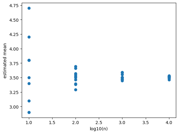
The law of large numbers states that the sample mean converges to the expected value as the sample size increases.
# In each experiment, we draw n samples and estimate the mean.
# For small n, each estimation might have large variability for different repetitions.
# As n increases, the variability decreases.
# For very large n, the estimates are almost the same as the true mean and the variability is very small.

# use n sample to estimate the mean
n = [10,100,1000,10000]

# number of repetitions for each n
k = 10

# store the estimates, each row is a different n, each column is a different repetition
estiamtes = np.zeros((len(n), k))

# sample sizes
logn = [] # log10 of n
means = [] # estimated mean

for ni in n:
    for k in range(10):
        x = np.random.randint(1, 7, ni)
        logn.append(np.log10(ni))
        means.append(np.mean(x))

fig, ax = plt.subplots()
# scatter plot of
ax.scatter(logn, means)
ax.set_xlabel('log10(n)')
ax.set_ylabel('estimated mean')
Text(0, 0.5, 'estimated mean')
Estimation of variance#
By definition the variance of a random variable X is defined as $\( \text{Var}(X) = E[(X - E[X])^2]\)$
We can estimate the variance by
We essentially replace the expected value with the sample mean.
# estimate variance of dice row
n = 100
x = np.random.randint(1, 7, n)
var1 = np.var(x)
var2 = np.mean((x - x.mean())**2)
print(var1, var2)
2.4059 2.4059
Correlation#
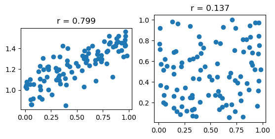
n = 100 # sample size

# X is a random variable uniformly distributed on [0, 1]
x = np.random.rand(n)

# Y is a linear function of X plus noise
y = 0.5*x+1 + np.random.normal(0, 0.1, n)

# z is independent of X
z = np.random.rand(n)


# compute our own correlation coefficient
# corr(x,y) = cov(x,y) / (std(x) * std(y))

my_corr = lambda x, y: np.mean((x - x.mean()) * (y - y.mean()))/(np.std(x) * np.std(y))
print(my_corr(x, y))

# using numpy
# np.corrcoef returns a matrix M with the correlation coefficients [corr(x,x), corr(x,y); corr(y,x), corr(y,y)]
corr_matrix = np.corrcoef(x, y)
print(corr_matrix)


# scatter plot
fig, ax = plt.subplots(1, 2)
ax[0].scatter(x, y)
ax[0].set_title(f'r = {my_corr(x, y):.3f}')
# equal axis
ax[0].set_aspect('equal')

ax[1].scatter(x, z)
ax[1].set_title(f'r = {my_corr(x, z):.3f}')
ax[1].set_aspect('equal')
0.7989815521783616
[[1.         0.79898155]
 [0.79898155 1.        ]]
Central limit theorem#
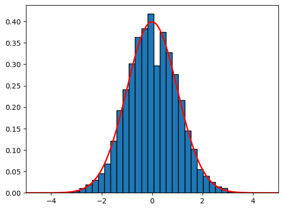
Roughly speaking, sample average are normally distributed for large sample sizes, regardless of the distribution of the underlying random variable!
This explains why the normal distribution is so common.
If \(X_1, X_2, \ldots, X_n\) are independent and identically distributed random variables with mean \(\mu\) and variance \(\sigma^2\), if we define $\( Z = \frac{\sqrt{n}(\bar{X} - \mu)}{\sigma}\)$ then for large n, Z is approximately normally distributed with mean 0 and variance 1.
# we know that the coin flip has a mean of 0.5 and a variance of 0.25
gaussian_density = lambda x,mu,sigma: (1/(sigma * np.sqrt(2 * np.pi)) * np.exp(- (x - mu)**2 / (2 * sigma**2)))

mu = 0.5
sigma = np.sqrt(0.25)

# number of experiments, in each experiment we draw n samples, and estimate the mean
N = 10000
n = 1000

z_samples = []


for i in range(N):

	# draw n samples
	x = np.random.randint(0, 2, n)
	# compute the sample mean
	sample_mean = np.mean(x)

	# do the transformation
	z = np.sqrt(n)*(sample_mean -  mu)/sigma

	z_samples.append(z)

# plot the histogram of z_samples
plt.hist(z_samples, bins=30, edgecolor='black', density=True)


# overlay the density function of the standard normal distribution
x = np.linspace(-10, 10, 1000)
y = gaussian_density(x, 0, 1)
plt.plot(x,y,linewidth=2, color='r')
plt.xlim(-5,5)
(-5.0, 5.0)
