Generative Adversarial Networks

So far we have seen exampels of supervised learning (such as regression and classification), unsupervised learning (such as clustering and dimensionality reduction).

In this notebook, we will explore generative models: models that generate new data that looks real.

As an example, we use the generate adversarial networks (GANs) to generate handwritten digits.

What is the function that we want to learn? In this case, we want to learn the mapping from a random noise vector to a handwritten digit.

The GANs are composed of two networks: the generator and the discriminator. The generator takes a random noise vector and generates a digit. The discriminator takes a digit and outputs the probability that the digit is real (i.e., it was drawn from the training set) or fake (i.e., it was generated by the generator).

That \(D\) be the discriminator and \(G\) be the generator (both are neural networks). The objective is

\[ \min_G \max_D V(D, G) = \mathbb{E}_{x \sim p_{\text{data}}(x)}[\log D(x)] + \mathbb{E}_{z \sim p_z(z)}[\log(1 - D(G(z)))] \]

where \(p_{\text{data}}(x)\) is the distribution of the real data and \(p_z(z)\) is the distribution of the noise vector.

This can be view as a game, where the generator tries to generate data that looks real and the discriminator tries to distinguish between real and fake data. If we look at the objective function,

• If the discriminator is good, the first term approaches 0. Because whatever G generates, D will predict 0 (is fake), therefore D(G(z)) is close to 0. And the second term approaches 0.

• If the generator is good, than D(G(z)) will predict 1 (is real). Therefore, the second term approaches \(-\infty\).

Therefore, we see D is trying to maximize the objective V and G is trying to minimize it.

# code adapted from https://github.com/lyeoni/pytorch-mnist-GAN
import os
import sys

import numpy as np
import torch
import torch.nn as nn
import torch.nn.parallel
import torch.backends.cudnn as cudnn
import torch.optim as optim
import torch.utils.data
import torchvision.transforms as transforms
import torchvision.datasets as dset
import torchvision.utils as vutils
import matplotlib.pyplot as plt

CUDA = True
DATA_PATH = './data'
BATCH_SIZE = 128
IMAGE_CHANNEL = 1
Z_DIM = 64
G_HIDDEN = 64
X_DIM = 64
D_HIDDEN = 64
EPOCH_NUM = 5
REAL_LABEL = 1
FAKE_LABEL = 0
lr = 2e-4
seed = 1

CUDA = CUDA and torch.cuda.is_available()
print("PyTorch version: {}".format(torch.__version__))
if CUDA:
    print("CUDA version: {}\n".format(torch.version.cuda))

if CUDA:
    torch.cuda.manual_seed(seed)
device = torch.device("cuda:0" if CUDA else "cpu")
cudnn.benchmark = True

PyTorch version: 2.1.0
CUDA version: 12.1

# Data preprocessing
dataset = dset.MNIST(root=DATA_PATH, download=False,
                     transform=transforms.Compose([
                     transforms.Resize(X_DIM),
                     transforms.ToTensor(),
                     transforms.Normalize((0.5,), (0.5,))
                     ]))

# Dataloader
dataloader = torch.utils.data.DataLoader(dataset, batch_size=BATCH_SIZE,
                                         shuffle=True, num_workers=2)

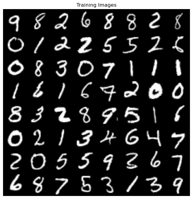
# Plot training images
real_batch = next(iter(dataloader))
plt.figure(figsize=(8,8))
plt.axis("off")
plt.title("Training Images")
plt.imshow(np.transpose(vutils.make_grid(real_batch[0].to(device)[:64], padding=2, normalize=True).cpu(),(1,2,0)))

<matplotlib.image.AxesImage at 0x7fe6a01568d0>

def weights_init(m):
    classname = m.__class__.__name__
    if classname.find('Conv') != -1:
        m.weight.data.normal_(0.0, 0.02)
    elif classname.find('BatchNorm') != -1:
        m.weight.data.normal_(1.0, 0.02)
        m.bias.data.fill_(0)

class Generator(nn.Module):
    def __init__(self):
        super(Generator, self).__init__()
        self.main = nn.Sequential(
            # input layer
            nn.ConvTranspose2d(Z_DIM, G_HIDDEN * 8, 4, 1, 0, bias=False),
            nn.BatchNorm2d(G_HIDDEN * 8),
            nn.ReLU(True),
            # 1st hidden layer
            nn.ConvTranspose2d(G_HIDDEN * 8, G_HIDDEN * 4, 4, 2, 1, bias=False),
            nn.BatchNorm2d(G_HIDDEN * 4),
            nn.ReLU(True),
            # 2nd hidden layer
            nn.ConvTranspose2d(G_HIDDEN * 4, G_HIDDEN * 2, 4, 2, 1, bias=False),
            nn.BatchNorm2d(G_HIDDEN * 2),
            nn.ReLU(True),
            # 3rd hidden layer
            nn.ConvTranspose2d(G_HIDDEN * 2, G_HIDDEN, 4, 2, 1, bias=False),
            nn.BatchNorm2d(G_HIDDEN),
            nn.ReLU(True),
            # output layer
            nn.ConvTranspose2d(G_HIDDEN, IMAGE_CHANNEL, 4, 2, 1, bias=False),
            nn.Tanh()
        )

    def forward(self, input):
        return self.main(input)

class Discriminator(nn.Module):
    def __init__(self):
        super(Discriminator, self).__init__()
        self.main = nn.Sequential(
            # 1st layer
            nn.Conv2d(IMAGE_CHANNEL, D_HIDDEN, 4, 2, 1, bias=False),
            nn.LeakyReLU(0.2, inplace=True),
            # 2nd layer
            nn.Conv2d(D_HIDDEN, D_HIDDEN * 2, 4, 2, 1, bias=False),
            nn.BatchNorm2d(D_HIDDEN * 2),
            nn.LeakyReLU(0.2, inplace=True),
            # 3rd layer
            nn.Conv2d(D_HIDDEN * 2, D_HIDDEN * 4, 4, 2, 1, bias=False),
            nn.BatchNorm2d(D_HIDDEN * 4),
            nn.LeakyReLU(0.2, inplace=True),
            # 4th layer
            nn.Conv2d(D_HIDDEN * 4, D_HIDDEN * 8, 4, 2, 1, bias=False),
            nn.BatchNorm2d(D_HIDDEN * 8),
            nn.LeakyReLU(0.2, inplace=True),
            # output layer
            nn.Conv2d(D_HIDDEN * 8, 1, 4, 1, 0, bias=False),
            nn.Sigmoid()
        )

    def forward(self, input):
        return self.main(input).view(-1, 1).squeeze(1)

# Create the generator
netG = Generator().to(device)
netG.apply(weights_init)
print(netG)

# Create the discriminator
netD = Discriminator().to(device)
netD.apply(weights_init)
print(netD)

Generator(
  (main): Sequential(
    (0): ConvTranspose2d(64, 512, kernel_size=(4, 4), stride=(1, 1), bias=False)
    (1): BatchNorm2d(512, eps=1e-05, momentum=0.1, affine=True, track_running_stats=True)
    (2): ReLU(inplace=True)
    (3): ConvTranspose2d(512, 256, kernel_size=(4, 4), stride=(2, 2), padding=(1, 1), bias=False)
    (4): BatchNorm2d(256, eps=1e-05, momentum=0.1, affine=True, track_running_stats=True)
    (5): ReLU(inplace=True)
    (6): ConvTranspose2d(256, 128, kernel_size=(4, 4), stride=(2, 2), padding=(1, 1), bias=False)
    (7): BatchNorm2d(128, eps=1e-05, momentum=0.1, affine=True, track_running_stats=True)
    (8): ReLU(inplace=True)
    (9): ConvTranspose2d(128, 64, kernel_size=(4, 4), stride=(2, 2), padding=(1, 1), bias=False)
    (10): BatchNorm2d(64, eps=1e-05, momentum=0.1, affine=True, track_running_stats=True)
    (11): ReLU(inplace=True)
    (12): ConvTranspose2d(64, 1, kernel_size=(4, 4), stride=(2, 2), padding=(1, 1), bias=False)
    (13): Tanh()
  )
)
Discriminator(
  (main): Sequential(
    (0): Conv2d(1, 64, kernel_size=(4, 4), stride=(2, 2), padding=(1, 1), bias=False)
    (1): LeakyReLU(negative_slope=0.2, inplace=True)
    (2): Conv2d(64, 128, kernel_size=(4, 4), stride=(2, 2), padding=(1, 1), bias=False)
    (3): BatchNorm2d(128, eps=1e-05, momentum=0.1, affine=True, track_running_stats=True)
    (4): LeakyReLU(negative_slope=0.2, inplace=True)
    (5): Conv2d(128, 256, kernel_size=(4, 4), stride=(2, 2), padding=(1, 1), bias=False)
    (6): BatchNorm2d(256, eps=1e-05, momentum=0.1, affine=True, track_running_stats=True)
    (7): LeakyReLU(negative_slope=0.2, inplace=True)
    (8): Conv2d(256, 512, kernel_size=(4, 4), stride=(2, 2), padding=(1, 1), bias=False)
    (9): BatchNorm2d(512, eps=1e-05, momentum=0.1, affine=True, track_running_stats=True)
    (10): LeakyReLU(negative_slope=0.2, inplace=True)
    (11): Conv2d(512, 1, kernel_size=(4, 4), stride=(1, 1), bias=False)
    (12): Sigmoid()
  )
)

# Initialize BCELoss function
criterion = nn.BCELoss()

# Create batch of latent vectors that I will use to visualize the progression of the generator
viz_noise = torch.randn(64, Z_DIM, 1, 1, device=device)

# Setup Adam optimizers for both G and D
optimizerD = optim.Adam(netD.parameters(), lr=lr, betas=(0.5, 0.999))
optimizerG = optim.Adam(netG.parameters(), lr=lr, betas=(0.5, 0.999))

# Training Loop

# Lists to keep track of progress
img_list = []
G_losses = []
D_losses = []
iters = 0

print("Starting Training Loop...")
for epoch in range(EPOCH_NUM):
    for i, data in enumerate(dataloader, 0):

        # (1) Update the discriminator with real data
        netD.zero_grad()
        # Format batch
        real_cpu = data[0].to(device)
        b_size = real_cpu.size(0)
        # all data are real
        label = torch.full((b_size,), REAL_LABEL, dtype=torch.float, device=device)
        # Forward pass real batch through D
        output = netD(real_cpu).view(-1)
        # Calculate loss on all-real batch
        errD_real = criterion(output, label)
        
        # Calculate gradients for D in backward pass
        errD_real.backward()
    

        # (2) Update the discriminator with fake data
        # Generate batch of latent vectors
        noise = torch.randn(b_size, Z_DIM, 1, 1, device=device)
        # Generate fake image batch with G
        fake = netG(noise)
        # all data are fake
        label.fill_(FAKE_LABEL)
        # Classify all fake batch with D
        output = netD(fake.detach()).view(-1)
        # Calculate D's loss on the all-fake batch
        errD_fake = criterion(output, label)
        # Calculate the gradients for this batch, accumulated (summed) with previous gradients
        errD_fake.backward()
        
        # Compute error of D as sum over the fake and the real batches
        errD = errD_real + errD_fake
        # Update D
        optimizerD.step()

        # (3) Update the generator with fake data
        netG.zero_grad()
        label.fill_(REAL_LABEL)  # fake labels are real for generator cost
        # Since we just updated D, perform another forward pass of all-fake batch through D
        output = netD(fake).view(-1)
        # Calculate G's loss based on this output
        errG = criterion(output, label)
        # Calculate gradients for G
        errG.backward()
        # Update G
        optimizerG.step()

        # Output training stats
        if i % 50 == 0:
            print('[%d/%d][%d/%d]\tLoss_D: %.4f\tLoss_G: %.4f'
                  % (epoch, EPOCH_NUM, i, len(dataloader), errD.item(), errG.item()))

        # Save Losses for plotting later
        G_losses.append(errG.item())
        D_losses.append(errD.item())

        # save the output on fixed noise
        if (iters % 500 == 0) or ((epoch == EPOCH_NUM-1) and (i == len(dataloader)-1)):
            with torch.no_grad():
                fake = netG(viz_noise).detach().cpu()
            img_list.append(vutils.make_grid(fake, padding=2, normalize=True))

        iters += 1

Starting Training Loop...
[0/5][0/469]	Loss_D: 1.9041	Loss_G: 5.0025
[0/5][50/469]	Loss_D: 0.0576	Loss_G: 6.8765
[0/5][100/469]	Loss_D: 0.1941	Loss_G: 4.6492
[0/5][150/469]	Loss_D: 0.2130	Loss_G: 3.9613
[0/5][200/469]	Loss_D: 0.1584	Loss_G: 4.1608
[0/5][250/469]	Loss_D: 0.1656	Loss_G: 4.0495
[0/5][300/469]	Loss_D: 0.0970	Loss_G: 3.2869
[0/5][350/469]	Loss_D: 0.1888	Loss_G: 3.8172
[0/5][400/469]	Loss_D: 0.1624	Loss_G: 3.6327
[0/5][450/469]	Loss_D: 0.3889	Loss_G: 2.8532
[1/5][0/469]	Loss_D: 0.2405	Loss_G: 3.0679
[1/5][50/469]	Loss_D: 0.4124	Loss_G: 3.7249
[1/5][100/469]	Loss_D: 0.3791	Loss_G: 3.4596
[1/5][150/469]	Loss_D: 0.3854	Loss_G: 2.4305
[1/5][200/469]	Loss_D: 0.3498	Loss_G: 2.8287
[1/5][250/469]	Loss_D: 0.8276	Loss_G: 3.6346
[1/5][300/469]	Loss_D: 0.9560	Loss_G: 1.2813
[1/5][350/469]	Loss_D: 0.8859	Loss_G: 1.1811
[1/5][400/469]	Loss_D: 0.4875	Loss_G: 1.4888
[1/5][450/469]	Loss_D: 0.4244	Loss_G: 1.6952
[2/5][0/469]	Loss_D: 0.3162	Loss_G: 2.3755
[2/5][50/469]	Loss_D: 0.2697	Loss_G: 2.8633
[2/5][100/469]	Loss_D: 0.5163	Loss_G: 1.6036
[2/5][150/469]	Loss_D: 0.2994	Loss_G: 2.2074
[2/5][200/469]	Loss_D: 0.4762	Loss_G: 1.6189
[2/5][250/469]	Loss_D: 0.3489	Loss_G: 2.2306
[2/5][300/469]	Loss_D: 0.6146	Loss_G: 1.2654
[2/5][350/469]	Loss_D: 1.2079	Loss_G: 0.8515
[2/5][400/469]	Loss_D: 0.3912	Loss_G: 3.1907
[2/5][450/469]	Loss_D: 1.0029	Loss_G: 2.2589
[3/5][0/469]	Loss_D: 0.3953	Loss_G: 2.6740
[3/5][50/469]	Loss_D: 0.6727	Loss_G: 6.6187
[3/5][100/469]	Loss_D: 0.2410	Loss_G: 3.0774
[3/5][150/469]	Loss_D: 1.1077	Loss_G: 0.7352
[3/5][200/469]	Loss_D: 0.1740	Loss_G: 4.0284
[3/5][250/469]	Loss_D: 1.8978	Loss_G: 0.6392
[3/5][300/469]	Loss_D: 0.3716	Loss_G: 2.4205
[3/5][350/469]	Loss_D: 0.2653	Loss_G: 3.0417
[3/5][400/469]	Loss_D: 0.3524	Loss_G: 4.1880
[3/5][450/469]	Loss_D: 0.2952	Loss_G: 3.1527
[4/5][0/469]	Loss_D: 0.3757	Loss_G: 3.1306
[4/5][50/469]	Loss_D: 1.0798	Loss_G: 3.5094
[4/5][100/469]	Loss_D: 0.3658	Loss_G: 1.6030
[4/5][150/469]	Loss_D: 0.0985	Loss_G: 3.9687
[4/5][200/469]	Loss_D: 0.6344	Loss_G: 2.5889
[4/5][250/469]	Loss_D: 0.6422	Loss_G: 2.3609
[4/5][300/469]	Loss_D: 1.2692	Loss_G: 6.5007
[4/5][350/469]	Loss_D: 0.2747	Loss_G: 2.6370
[4/5][400/469]	Loss_D: 0.2975	Loss_G: 3.3537
[4/5][450/469]	Loss_D: 0.5319	Loss_G: 2.0657

# Save the model
torch.save(netG.state_dict(), 'generator.pth')
torch.save(netD.state_dict(), 'discriminator.pth')

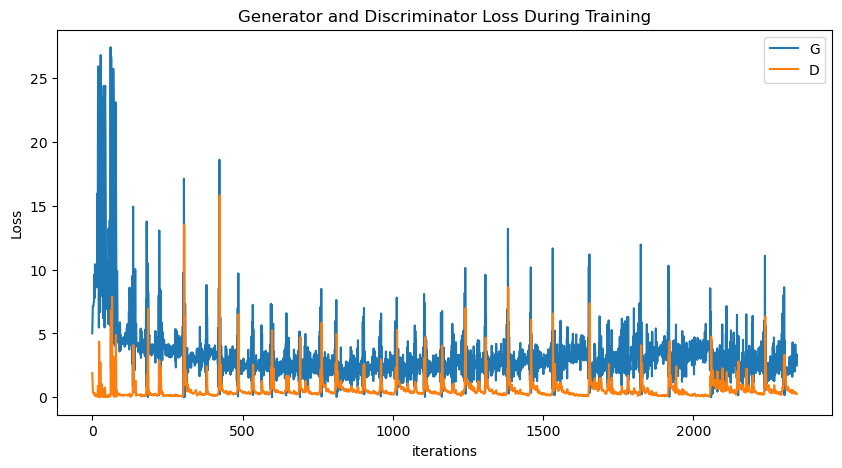
plt.figure(figsize=(10,5))
plt.title("Generator and Discriminator Loss During Training")

# plot in log scale
plt.plot(G_losses,label="G")
plt.plot(D_losses,label="D")

plt.xlabel("iterations")
plt.ylabel("Loss")
plt.legend()
plt.show()

import matplotlib.pyplot as plt
import matplotlib.animation as animation
from IPython.display import HTML
import torch

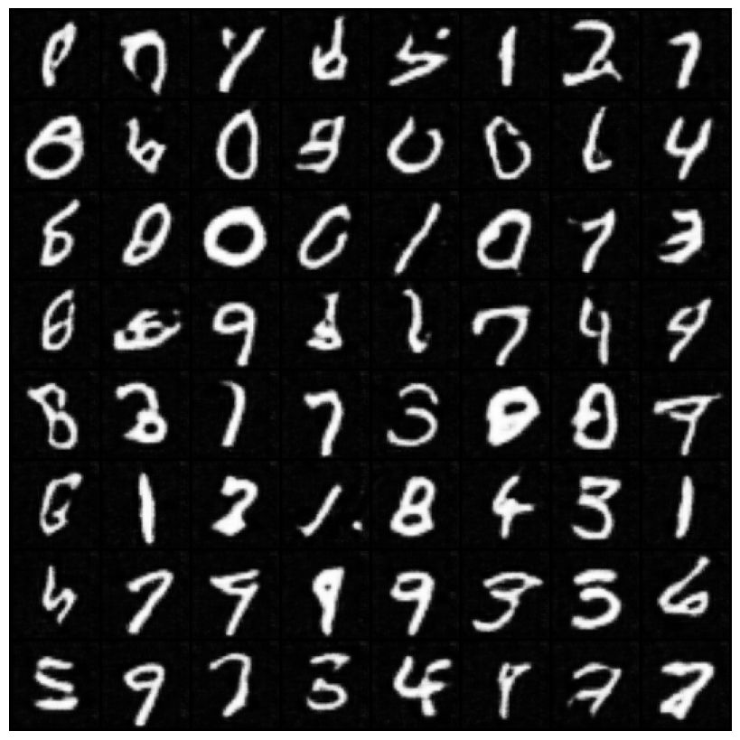
fig = plt.figure(figsize=(10,8))

# Adjust the subplots to reduce padding
fig.subplots_adjust(left=0, right=1, top=1, bottom=0)

plt.axis("off")
ims = [[plt.imshow(i.permute(1,2,0), animated=True)] for i in img_list]

ani = animation.ArtistAnimation(fig, ims, interval=1000, repeat_delay=1000, blit=True)
HTML(ani.to_jshtml())

Once Loop Reflect

Generative AI holds immense potential. However, its capabilities also raise concerns:

Generative AI Has an Intellectual Property Problem

Humans are biased. Generative AI is even worse

Election disinformation takes a big leap with AI being used to deceive worldwide