OOP and Gradient Descent#
Class and Object#
A class combines data/attribute and functionality/method together
An object is an instance of a class
from math import sqrt

class Vector():
    # custom type for 2d vectors

    # class attribute shared by all objects of this class
    dim = 2

    def __init__(self, input_x, input_y):
        # constructor, called when new object is created, Vector(x,y)
        # self is the object being created
        # .x and .y are object attributes
        self.x = input_x
        self.y = input_y

    def length(self):
        # length method, returns length of vector
        l = sqrt(self.x**2+self.y**2)
        return l

    def scale(self, c):
        # method that scales the vector by a constant c
        # changes the object itself
        # no return value, so returns None
        self.x = self.x * c
        self.y = self.y * c

    def __repr__(self):
        # string representation of the object
        # without this method, it prints the memory address
        return f'({self.x},{self.y})'


    def add(self, other_vector):
        # method that adds another vector to this vector, returns new vector
        x_new = self.x + other_vector.x
        y_new = self.y + other_vector.y
        return Vector(x_new, y_new)

    def __add__(self, other_vector):
        # special method that overloads the + operator
        # without this method, vector + vector would raise an error
        x_new = self.x + other_vector.x
        y_new = self.y + other_vector.y
        return Vector(x_new, y_new)

    def normalize(self):
        # method that scales the vector to unit length
        # can call other methods of the same object
        l = self.length()
        self.scale(1/l)
v = Vector(3,4)
v.x
print(v.x)
v.normalize()
print(v.length())
print(v)
3
1.0
(0.6000000000000001,0.8)
v = Vector(1,1)
w = Vector(2,3)

# custom add method
p = v.add(w)
print(p)

# this is actually calling the __add__ method
q = v + w
print(q)
(3,4)
(3,4)
Gradient Descent (GD)#
Problem: minimize f(x), \(x \in \mathbb{R}^d\)
Suppose \(\nabla f(x) = [f'(x_1), f'(x_2), ... , f'(x_d)]^T\) is the gradient of the function \(f(x)\) at point \(x\), and we have some initial guess \(x_0\).
Our goal is to generate a sequence of numbers \(x_0\), \(x_1\), \(x_2\) … that iteratively approaches a local minimizer of the function.
Idea: the gradient of a function at a point gives the direction of the steepest ascent of the function at that point. So, if we move in the opposite direction of the gradient, we should be moving towards a local minimum.
where \(\alpha\) is the step size or learning rate. We repeat this process until \(|f'(x_i)|\) is close to 0 for some \(i\).
Note:
This algorithm tends to go to the closest local minimum.
If \(\nabla f(x_i)=0\), then we are at stationary point so we won’t move.
In the simplest form \(\alpha\) is fixed by the user. For more advanced versions, it will be adaptive or randomized.
Interactive Visualization#
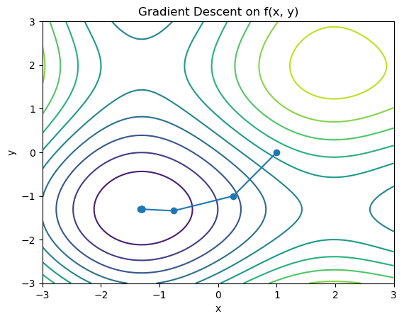
Implementing GD using the Vector class#
import numpy as np
import matplotlib.pyplot as plt


# test function 1, simple quadratic
# f = lambda x, y: x**2 + y**2
# grad_f = lambda x, y: Vector(2 * x , 2 * y)

# test function 2, more complex landscape
f = lambda x, y: x**2 + y**2 + 10 * np.sin(x) + 10 * np.sin(y)
grad_f = lambda x, y: Vector(2 * x + 10 * np.cos(x), 2 * y + 10 * np.cos(y))

# initial guess and learning rate, this is x0
xi = Vector(1,0)
learning_rate = 0.1
trajectory = [xi]
n_steps = 10

# Gradient descent algorithm
for _ in range(n_steps):  # Fewer iterations for clarity

    # compute gradient vector
    grad = grad_f(xi.x, xi.y)

    # this is -learning_rate * grad
    grad.scale(-learning_rate)

    # this is x_{i+1} = x_i  - learning_rate * grad
    xi = xi + grad

    # append new point to trajectory
    trajectory.append(xi)

# why not write "xi - learning_rate * grad" ?
# because our custom class does not define subtraction and multiplication
# we only defined addition and scaling


### the following code is for visualizing the contour of the objective function f(x,y)
# see the documentation and example for contour plot
# https://matplotlib.org/stable/gallery/images_contours_and_fields/contour_demo.html#sphx-glr-gallery-images-contours-and-fields-contour-demo-py
# Create a grid of x, y trajectory for the contour plot
x = np.linspace(-3, 3, 400)
y = np.linspace(-3, 3, 400)
X, Y = np.meshgrid(x, y)
Z = f(X, Y)
# Contour plot
plt.contour(X, Y, Z, levels=10)  # Adjust the number of levels for more detail
### end of plotting contour

# plot trajectory
x_coords = [p.x for p in trajectory]
y_coords = [p.y for p in trajectory]
plt.plot(x_coords, y_coords, '-o')

plt.title('Gradient Descent on f(x, y)')
plt.xlabel('x')
plt.ylabel('y')
plt.show()

# print final objective value and final point
print(f'Final objective value: {f(xi.x, xi.y)} at point {xi}')

Final objective value: -15.891646751230518 at point (-1.306439918487552,-1.3064400276166004)