Logistic Regression for Multiclass Classification

In this part, we consider logistic regression for K > 2 classes. We have data \((\mathbf{x}_i, y_i)\) for i = 1, 2, …, N, where \(\mathbf{x}_i\in\mathbb{R}^p\) is the input/feature and \(y_i\) is the output/label, which indicates the class of the input.

We treat the output \(y_i\) as a categorical variable, which indicates the class of the input.

Model

We consider the augmented data \(\mathbf{x}_i = [1, x_{i1}, x_{i2}, ..., x_{ip}]\) for i = 1, 2, …, N, where \(x_{ij}\) is the j-th feature of the i-th input, and we assume that the output \(y_i\) can take K different values, 1, …, K

We assume the the probability of the input \(\mathbf{x}\) belonging to class 1 to K is given by a vector of probabilities.

\[\begin{split} f(\mathbf{x}; \mathbf{W}) = \begin{bmatrix} f_1(\mathbf{x}; \mathbf{W}) \\ f_2(\mathbf{x}; \mathbf{W}) \\ \vdots \\ f_K(\mathbf{x}; \mathbf{W}) \end{bmatrix} = \frac{1}{\sum_{k=1}^K \exp(\mathbf{w}_k^T\mathbf{x})} \begin{bmatrix} \exp(\mathbf{w}_1^T\mathbf{x}) \\ \exp(\mathbf{w}_2^T\mathbf{x}) \\ \vdots \\ \exp(\mathbf{w}_K^T\mathbf{x}) \end{bmatrix} \end{split}\]

• \(\mathbf{w}_i = [w_{i0}, w_{i1}, w_{i2}, ..., w_{ip}]\) is the \(p+1\) dimensional vector of coefficients for class \(i\)

• \(f_j(\mathbf{x};\mathbf{W})\) is the probability of the input \(\mathbf{x}\) belonging to class j. By construction, \(\sum_{j=1}^K f_j(\mathbf{x}; \mathbf{W}) = 1\) for all \(\mathbf{x}\). That is, the probabilities of the input \(\mathbf{x}\) belonging to class 1 to K sum to 1.

• \(\mathbf{W}\) is the matrix of all the coefficients \(\mathbf{w}_i\) for i = 1, 2, …, K.

\[\begin{split} \mathbf{W} = \begin{bmatrix} \mathbf{w}_1^T \\ \mathbf{w}_2^T \\ \vdots \\ \mathbf{w}_K^T \end{bmatrix} = \begin{bmatrix} w_{10} & w_{11} & \cdots & w_{1p} \\ w_{20} & w_{21} & \cdots & w_{2p} \\ \vdots & \vdots & \ddots & \vdots \\ w_{K0} & w_{K1} & \cdots & w_{Kp} \end{bmatrix} \end{split}\]

where \(w_{ij}\) is the j-th coefficient for class i.

Cross-entropy loss

Define the indicator variable \(y_{ik}\) as

\[\begin{split} y_{ik} = \begin{cases} 1 & \text{if } y_i \text{ is class k} \\ 0 & \text{otherwise} \end{cases} \end{split}\]

Essentiall, we encode the categorical variable \(y_{i}\) as a vector in \(\mathbb{R}^K\) with a 1 at the k-th position and 0 elsewhere.

The cross-entropy loss is given by

\[ L(\mathbf{W}) = -\sum_{i=1}^N \sum_{k=1}^K y_{ik}\log(f_k(\mathbf{x}_i; \mathbf{W})) \]

And the optimal weight matrix \(\mathbf{W}\) is obtained by minimizing the loss function \(L(\mathbf{W})\).

Exercises: show that when K=2, this reduces to the binary logistic regression loss.

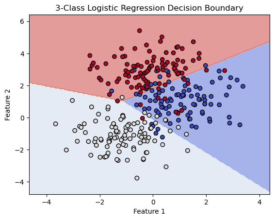
Visualization

import matplotlib.pyplot as plt
import numpy as np
from sklearn.linear_model import LogisticRegression
from sklearn.inspection import DecisionBoundaryDisplay

# Set random seed for reproducibility
np.random.seed(0)

# Number of samples per class
N = 100

# Generate data for three classes, each class has a different mean
x_class1 = np.random.multivariate_normal([1, 1], np.eye(2), N)
x_class2 = np.random.multivariate_normal([-1, -1], np.eye(2), N)
x_class3 = np.random.multivariate_normal([0, 3], np.eye(2), N)

# Combine into a single dataset
X = np.vstack((x_class1, x_class2, x_class3))
y = np.concatenate((np.zeros(N), np.ones(N), 2*np.ones(N)))

# Create a logistic regression classifier with multinomial option for multi-class
clf = LogisticRegression(multi_class='multinomial', solver='lbfgs', max_iter=1000)
clf.fit(X, y)

# Plot the decision boundaries using DecisionBoundaryDisplay
fig, ax = plt.subplots()
db_display = DecisionBoundaryDisplay.from_estimator(
    clf,
    X,
    grid_resolution=200,
    response_method="predict",  # Can be "predict_proba" for probability contours
    cmap='coolwarm',
    alpha=0.5,
    ax=ax
)
# Scatter plot of the data points
scatter = ax.scatter(X[:, 0], X[:, 1], c=y, edgecolors='k', cmap='coolwarm')

# Adding title and labels
ax.set_title('3-Class Logistic Regression Decision Boundary')
ax.set_xlabel('Feature 1')
ax.set_ylabel('Feature 2')

# Show plot
plt.show()

Classification using penguins dataset

import pandas as pd
import seaborn as sns
from sklearn.model_selection import train_test_split
from sklearn.linear_model import LogisticRegression
from sklearn.preprocessing import LabelEncoder
from sklearn.metrics import accuracy_score, confusion_matrix
import matplotlib.pyplot as plt
from sklearn.preprocessing import StandardScaler


# Load the dataset
df = sns.load_dataset('penguins')

# Drop rows with missing values
df.dropna(subset=['bill_length_mm', 'bill_depth_mm', 'flipper_length_mm', 'body_mass_g'], inplace=True)


features = ['bill_length_mm', 'bill_depth_mm', 'flipper_length_mm', 'body_mass_g']

# scale the features
scaler = StandardScaler()
df[features] = scaler.fit_transform(df[features])

# Select features
X = df[features]
y = df['species']

# Split the data into training and testing sets
X_train, X_test, y_train, y_test = train_test_split(X, y, test_size=0.25, random_state=0)

# Initialize and train the logistic regression model
clf = LogisticRegression(penalty=None)
clf.fit(X_train, y_train)

# Calculate the training and test accuracy
score_train = clf.score(X_train, y_train)
score_test = clf.score(X_test, y_test)
print(f"Training accuracy: {score_train:.2f}")
print(f"Test accuracy: {score_test:.2f}")


# Predict on the test set
y_pred = clf.predict(X_test)

# Evaluate the model
conf_matrix = confusion_matrix(y_test, y_pred)
print("Confusion Matrix:\n", conf_matrix)

# Plotting the confusion matrix
sns.heatmap(conf_matrix, annot=True, fmt='d', cmap='Blues', xticklabels=le.classes_, yticklabels=le.classes_)
plt.xlabel('Predicted Labels')
plt.ylabel('True Labels')
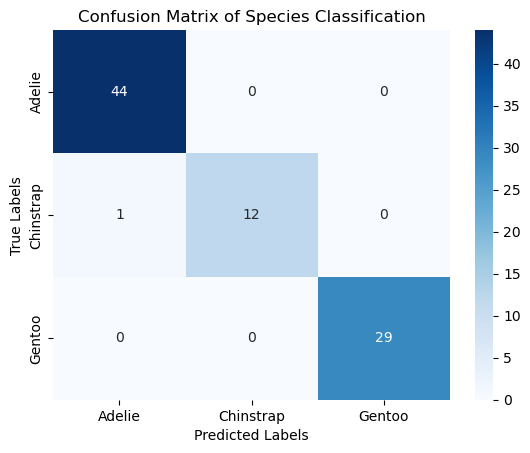
plt.title('Confusion Matrix of Species Classification')
plt.show()

Training accuracy: 1.00
Test accuracy: 0.99
Confusion Matrix:
 [[44  0  0]
 [ 1 12  0]
 [ 0  0 29]]