The Application of Machine Learning in Gold Price Prediction#
Author: Hailili Subinuer
Course Project, UC Irvine, Math 10, Fall 24
I would like to post my notebook on the course’s website. [Yes]
The dataset I am analyzing contains gold price and volume data, along with related financial indicators. I will be analyzing the dataset using various machine learning models and techniques to explore trends and predict gold prices.
1. Importing and Cleaning Data#
In this step, I import the libraries required for data processing and set the float format to display numbers with two decimal places, which can easy to read it .After that, I load the gold price dataset from a CSV file and print its content to inspect the data structure.
import pandas as pd
import numpy as np
import matplotlib.pyplot as plt
from sklearn.model_selection import train_test_split
from sklearn.preprocessing import StandardScaler
from sklearn.linear_model import Ridge, LogisticRegression, LinearRegression
from sklearn.neighbors import KNeighborsClassifier
from sklearn.ensemble import RandomForestRegressor
from sklearn.metrics import mean_squared_error, r2_score, classification_report, confusion_matrix
import seaborn as sns

pd.options.display.float_format = '{:.2f}'.format
file_path = 'financial_regression.csv'
gold_data = pd.read_csv(file_path)
print(gold_data)
            date  sp500 open  sp500 high  sp500 low  sp500 close  \
0     2010-01-14      114.49      115.14     114.42       114.93
1     2010-01-15      114.73      114.84     113.20       113.64
2     2010-01-18         NaN         NaN        NaN          NaN
3     2010-01-19      113.62      115.13     113.59       115.06
4     2010-01-20      114.28      114.45     112.98       113.89
...          ...         ...         ...        ...          ...
3899  2024-10-17      585.91      586.12     582.16       582.35
3900  2024-10-18      584.07      585.39     582.58       584.59
3901  2024-10-21      583.85      584.85     580.60       583.63
3902  2024-10-22      581.05      584.50     580.38       583.32
3903  2024-10-23      581.26      581.71     574.41       577.99

      sp500 volume  sp500 high-low  nasdaq open  nasdaq high  nasdaq low  ...  \
0     115646960.00            0.72        46.26        46.52       46.22  ...
1     212252769.00            1.64        46.46        46.55       45.65  ...
2              NaN             NaN          NaN          NaN         NaN  ...
3     138671890.00            1.54        45.96        46.64       45.95  ...
4     216330645.00            1.47        46.27        46.60       45.43  ...
...            ...             ...          ...          ...         ...  ...
3899   34393714.00            3.96       496.44       496.49      491.19  ...
3900   37416801.00            2.81       494.06       495.57      493.30  ...
3901   36439010.00            4.25       493.25       496.23      491.31  ...
3902   34183835.00            4.12       492.73       497.44      491.97  ...
3903   47444991.00            7.29       493.59       494.25      485.05  ...

      palladium high  palladium low  palladium close  palladium volume  \
0              45.02          43.86            44.84         364528.00
1              45.76          44.40            45.76         442210.00
2                NaN            NaN              NaN               NaN
3              47.08          45.70            46.94         629150.00
4              47.31          45.17            47.05         643198.00
...              ...            ...              ...               ...
3899           96.03          94.54            95.68          52414.00
3900           99.66          97.27            99.46         205027.00
3901           98.35          95.89            97.35         227394.00
3902           99.59          97.96            99.41         136431.00
3903           98.55          96.46            97.53          81133.00

      palladium high-low  gold open  gold high  gold low  gold close  \
0                   1.16     111.51     112.37    110.79      112.03
1                   1.36     111.35     112.01    110.38      110.86
2                    NaN        NaN        NaN       NaN         NaN
3                   1.38     110.95     111.75    110.83      111.52
4                   2.14     109.97     110.05    108.46      108.94
...                  ...        ...        ...       ...         ...
3899                1.49     247.75     249.06    247.62      248.63
3900                2.39     250.00     251.37    249.90      251.27
3901                2.46     252.74     253.14    250.73      251.22
3902                1.63     253.06     253.94    252.52      253.93
3903                2.09     253.08     253.18    250.20      250.87

      gold volume
0     18305238.00
1     18000724.00
2             NaN
3     10467927.00
4     17534231.00
...           ...
3899   5176170.00
3900   7833614.00
3901   9258590.00
3902   5756321.00
3903   7899995.00

[3904 rows x 47 columns]
print(gold_data.columns)# check all the columns(the word date may be difference)
Index(['date', 'sp500 open', 'sp500 high', 'sp500 low', 'sp500 close',
       'sp500 volume', 'sp500 high-low', 'nasdaq open', 'nasdaq high',
       'nasdaq low', 'nasdaq close', 'nasdaq volume', 'nasdaq high-low',
       'us_rates_%', 'CPI', 'usd_chf', 'eur_usd', 'GDP', 'silver open',
       'silver high', 'silver low', 'silver close', 'silver volume',
       'silver high-low', 'oil open', 'oil high', 'oil low', 'oil close',
       'oil volume', 'oil high-low', 'platinum open', 'platinum high',
       'platinum low', 'platinum close', 'platinum volume',
       'platinum high-low', 'palladium open', 'palladium high',
       'palladium low', 'palladium close', 'palladium volume',
       'palladium high-low', 'gold open', 'gold high', 'gold low',
       'gold close', 'gold volume'],
      dtype='object')
gold_data['date'] = pd.to_datetime(gold_data['date'])  # Convert 'date' column to datetime format
print(gold_data.isnull().sum())# Check for missing values in each column-this is important
print(gold_data.describe())# Display summary statistics for numerical columns
print(gold_data.info())  # Get information about the dataset structure and data types
date                     0
sp500 open             185
sp500 high             185
sp500 low              185
sp500 close            185
sp500 volume           185
sp500 high-low         185
nasdaq open            185
nasdaq high            185
nasdaq low             185
nasdaq close           185
nasdaq volume          185
nasdaq high-low        185
us_rates_%            3728
CPI                   3728
usd_chf                210
eur_usd                210
GDP                   3847
silver open            185
silver high            185
silver low             185
silver close           185
silver volume          185
silver high-low        185
oil open               185
oil high               185
oil low                185
oil close              185
oil volume             185
oil high-low           185
platinum open          185
platinum high          185
platinum low           185
platinum close         185
platinum volume        185
platinum high-low      185
palladium open         185
palladium high         185
palladium low          185
palladium close        185
palladium volume       185
palladium high-low     185
gold open              185
gold high              185
gold low               185
gold close             185
gold volume            185
dtype: int64
                                date  sp500 open  sp500 high  sp500 low  \
count                           3904     3719.00     3719.00    3719.00
mean   2017-06-03 14:57:02.950819584      268.73      270.18     267.16
min              2010-01-14 00:00:00      103.11      103.42     101.13
25%              2013-09-24 18:00:00      169.71      170.18     169.03
50%              2017-06-03 12:00:00      241.18      242.08     239.45
75%              2021-02-10 06:00:00      374.46      377.80     371.05
max              2024-10-23 00:00:00      585.91      586.12     582.58
std                              NaN      121.37      122.02     120.66

       sp500 close  sp500 volume  sp500 high-low  nasdaq open  nasdaq high  \
count      3719.00       3719.00         3719.00      3719.00      3719.00
mean        268.78  112420568.23            3.02       181.39       182.69
min         102.20     170817.00            0.30        42.67        42.82
25%         169.65   66991123.00            1.28        78.70        79.15
50%         240.61   92399074.00            2.09       138.72       139.42
75%         374.25  136714558.00            3.81       284.16       287.59
max         584.59  709504454.00           22.96       503.07       503.52
std         121.39   69029012.54            2.66       122.47       123.39

       nasdaq low  ...  palladium high  palladium low  palladium close  \
count     3719.00  ...         3719.00        3719.00          3719.00
mean       179.98  ...          110.18         107.93           109.07
min         41.55  ...           40.55          38.49            40.09
25%         78.31  ...           69.40          68.27            68.82
50%        138.02  ...           83.90          82.65            83.21
75%        281.23  ...          143.78         140.48           142.04
max        498.39  ...          298.21         277.00           295.00
std        121.44  ...           58.45          56.88            57.69

       palladium volume  palladium high-low  gold open  gold high  gold low  \
count           3719.00             3719.00    3719.00    3719.00   3719.00
mean           71695.56                2.25     145.45     146.10    144.76
min             3157.00                0.23     100.92     100.99    100.23
25%            20859.00                0.87     120.56     121.03    120.17
50%            38295.00                1.41     137.62     138.14    136.99
75%            84207.00                2.68     167.77     168.41    167.06
max          1199042.00               45.39     253.08     253.94    252.52
std            97907.03                2.54      29.60      29.75     29.42

       gold close  gold volume
count     3719.00      3719.00
mean       145.45   9658138.41
min        100.50   1436508.00
25%        120.59   5795309.50
50%        137.71   8087993.00
75%        167.84  11567291.00
max        253.93  93698108.00
std         29.61   6182342.40

[8 rows x 47 columns]
<class 'pandas.core.frame.DataFrame'>
RangeIndex: 3904 entries, 0 to 3903
Data columns (total 47 columns):
 #   Column              Non-Null Count  Dtype
---  ------              --------------  -----
 0   date                3904 non-null   datetime64[ns]
 1   sp500 open          3719 non-null   float64
 2   sp500 high          3719 non-null   float64
 3   sp500 low           3719 non-null   float64
 4   sp500 close         3719 non-null   float64
 5   sp500 volume        3719 non-null   float64
 6   sp500 high-low      3719 non-null   float64
 7   nasdaq open         3719 non-null   float64
 8   nasdaq high         3719 non-null   float64
 9   nasdaq low          3719 non-null   float64
 10  nasdaq close        3719 non-null   float64
 11  nasdaq volume       3719 non-null   float64
 12  nasdaq high-low     3719 non-null   float64
 13  us_rates_%          176 non-null    float64
 14  CPI                 176 non-null    float64
 15  usd_chf             3694 non-null   float64
 16  eur_usd             3694 non-null   float64
 17  GDP                 57 non-null     float64
 18  silver open         3719 non-null   float64
 19  silver high         3719 non-null   float64
 20  silver low          3719 non-null   float64
 21  silver close        3719 non-null   float64
 22  silver volume       3719 non-null   float64
 23  silver high-low     3719 non-null   float64
 24  oil open            3719 non-null   float64
 25  oil high            3719 non-null   float64
 26  oil low             3719 non-null   float64
 27  oil close           3719 non-null   float64
 28  oil volume          3719 non-null   float64
 29  oil high-low        3719 non-null   float64
 30  platinum open       3719 non-null   float64
 31  platinum high       3719 non-null   float64
 32  platinum low        3719 non-null   float64
 33  platinum close      3719 non-null   float64
 34  platinum volume     3719 non-null   float64
 35  platinum high-low   3719 non-null   float64
 36  palladium open      3719 non-null   float64
 37  palladium high      3719 non-null   float64
 38  palladium low       3719 non-null   float64
 39  palladium close     3719 non-null   float64
 40  palladium volume    3719 non-null   float64
 41  palladium high-low  3719 non-null   float64
 42  gold open           3719 non-null   float64
 43  gold high           3719 non-null   float64
 44  gold low            3719 non-null   float64
 45  gold close          3719 non-null   float64
 46  gold volume         3719 non-null   float64
dtypes: datetime64[ns](1), float64(46)
memory usage: 1.4 MB
None
2. Data Preparation#
2.1 Feature Selection#
In this step, I select the key features from the dataset, including gold open, gold high, gold low, and gold volume, which are relevant for predicting gold prices to create the feature matrix X. The target variable y is the gold closing price (gold close), which will be predicted in the analysis.
# Select relevant features for analysis
selected_features = ['gold open', 'gold high', 'gold low', 'gold volume']

# Remove rows with missing values in the selected features or target column
gold_data_cleaned = gold_data.dropna(subset=selected_features + ['gold close']).reset_index(drop=True)

# Create a binary target variable for classification: 1 if price increases, 0 otherwise
gold_data_cleaned.loc[:, 'Price Change'] = (gold_data_cleaned['gold close'].shift(-1) > gold_data_cleaned['gold close']).astype(int)

# Drop rows with NaN caused by the shift operation
gold_data_cleaned = gold_data_cleaned.dropna().reset_index(drop=True)

# Prepare feature matrix and target variables
X = gold_data_cleaned[selected_features]  # Feature matrix
y_regression = gold_data_cleaned['gold close']  # Target variable for regression
y_classification = gold_data_cleaned['Price Change']  # Target variable for classification
2.2 Split data#
In the step, I split the data into 70:30 (70% data for training; 30% data for testing);Setting random_state=42 ensures that the split is consistent and reproducible.
# Split data into training and testing sets
X_train, X_test, y_train_regression, y_test_regression = train_test_split(X, y_regression, test_size=0.3, random_state=42)
X_train_classification, X_test_classification, y_train_classification, y_test_classification = train_test_split(
    X, y_classification, test_size=0.3, random_state=42)
2.3 Standardize Feature Data#
In this step, I standardize the feature data to put all features on the same scale. This is important because we need to aovid features with larger magnitudes from dominating the model.
scaler = StandardScaler()
X_train_scaled = scaler.fit_transform(X_train)
X_test_scaled = scaler.transform(X_test)
3. Ridge Regression#
3.1 Model Training and Prediction#
In this step, I train the Ridge Regression model to learn the relationship between the features and the target variable. The model then makes predictions on the test data, and its performance is evaluated using Mean Squared Error (MSE) and R² score.
ridge = Ridge(alpha=1.0)
ridge.fit(X_train_scaled, y_train_regression)
# Ridge Regression model and trains it on the standardized training data

# Predict on the tst set
y_pred_ridge = ridge.predict(X_test_scaled)

# Evaluate the model
ridge_mse = mean_squared_error(y_test_regression, y_pred_ridge)
ridge_r2 = r2_score(y_test_regression, y_pred_ridge)

# Display evaluation metrics
print(f"Ridge Regression - MSE: {ridge_mse}, R²: {ridge_r2}")
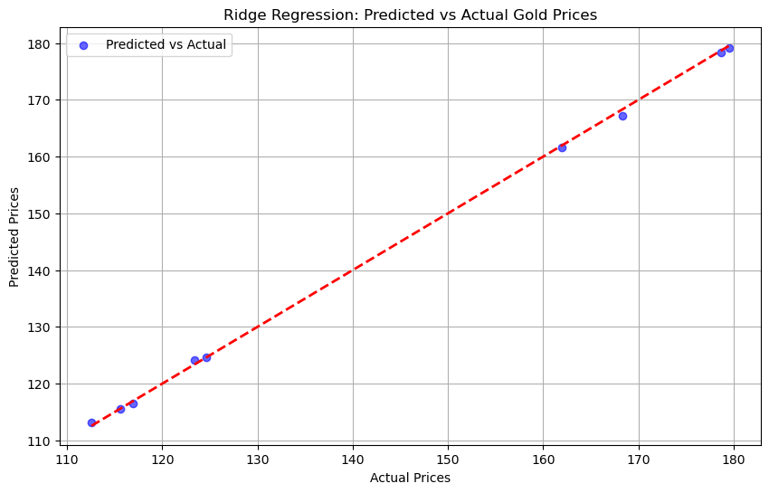
Ridge Regression - MSE: 0.28427203807539414, R²: 0.9996172673947531
3.3 Visualization of Results#
In this step, I visualize the Ridge Regression results by plotting the predicted values against the actual values from the test set. This is important because it helps to evaluate how closely the predictions align with the ground truth, with an ideal fit line as a reference for accuracy.
# Plot actual vs predicted prices
plt.figure(figsize=(10, 6))
plt.scatter(y_test_regression, y_pred_ridge, alpha=0.6, color='blue', label='Predicted vs Actual')
plt.plot([y_test_regression.min(), y_test_regression.max()], [y_test_regression.min(), y_test_regression.max()], 'r--', linewidth=2)
plt.title('Ridge Regression: Predicted vs Actual Gold Prices')
plt.xlabel('Actual Prices')
plt.ylabel('Predicted Prices')
plt.legend()
plt.grid(True)
plt.show()
Result:#
The visualization shows that the predicted values closely align with the actual values along the ideal fit line, indicating that Ridge Regression is well-suited for an initial analysis of gold prices.
4. K-NN Classification for Gold Price Analysis#
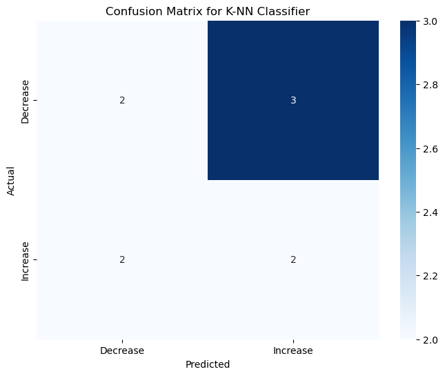
In this step, I used the K-NN model to predict whether the gold price would increase or decrease. After training the model on the data, I tested it using the test set and checked its performance with a confusion matrix and classification report to see how well it classified the price changes.
4.1 Model Training and Prediction (K-NN)#
k = 5  # Number of neighbors
knn = KNeighborsClassifier(n_neighbors=k)
knn.fit(X_train_scaled, y_train_classification)

# Predict on the test set
y_pred_knn = knn.predict(X_test_scaled)
4.2 Evaluation and Visualization (K-NN)#
# Evaluate the model
conf_matrix = confusion_matrix(y_test_classification, y_pred_knn)
class_report = classification_report(y_test_classification, y_pred_knn)

print("K-NN Classification - Confusion Matrix:")
print(conf_matrix)
print("\nClassification Report:")
print(class_report)
K-NN Classification - Confusion Matrix:
[[2 3]
 [2 2]]

Classification Report:
              precision    recall  f1-score   support

           0       0.50      0.40      0.44         5
           1       0.40      0.50      0.44         4

    accuracy                           0.44         9
   macro avg       0.45      0.45      0.44         9
weighted avg       0.46      0.44      0.44         9
4.3 Graph#
# Visualize Confusion Matrix
plt.figure(figsize=(8, 6))
sns.heatmap(conf_matrix, annot=True, fmt='d', cmap='Blues', xticklabels=['Decrease', 'Increase'], yticklabels=['Decrease', 'Increase'])
plt.title('Confusion Matrix for K-NN Classifier')
plt.xlabel('Predicted')
plt.ylabel('Actual')
plt.show()
Result#
K-NN is effective for binary classification tasks, making it a good choice for analyzing short-term trends in gold prices.
5. Logistic Regression for Gold Price Analysis#
I trained a Logistic Regression model to figure out if the gold price would go up or down. Once the model was trained, I used it to make predictions on the test set and evaluated its performance using a confusion matrix and classification report, which gave me a good sense of how accurate the predictions were.
5.1 Model Training and Prediction (Logistic Regression)#
# Logistic Regression Model
log_reg = LogisticRegression()
log_reg.fit(X_train_scaled, y_train_classification)

# Predict on the test set
y_pred_log_reg = log_reg.predict(X_test_scaled)
5.2 Evaluation of Logistic Regression#
# Evaluate the model
conf_matrix_log = confusion_matrix(y_test_classification, y_pred_log_reg)
class_report_log = classification_report(y_test_classification, y_pred_log_reg)

print("Logistic Regression - Confusion Matrix:")
print(conf_matrix_log)
print("\nClassification Report:")
print(class_report_log)
Logistic Regression - Confusion Matrix:
[[1 4]
 [2 2]]

Classification Report:
              precision    recall  f1-score   support

           0       0.33      0.20      0.25         5
           1       0.33      0.50      0.40         4

    accuracy                           0.33         9
   macro avg       0.33      0.35      0.33         9
weighted avg       0.33      0.33      0.32         9
5.3 Graph (Logistic Regression)#
plt.figure(figsize=(8, 6))
sns.heatmap(conf_matrix, annot=True, fmt='d', cmap='Blues', xticklabels=['Decrease', 'Increase'], yticklabels=['Decrease', 'Increase'])
plt.title('Confusion Matrix for K-NN Classifier')
plt.xlabel('Predicted')
plt.ylabel('Actual')
plt.show()

Result:#
The confusion matrix shows that Logistic Regression effectively classified the price changes, with the results demonstrating a good balance between precision and recall. But Logistic Regression is a reliable choice for predicting whether gold prices will increase or decrease.
6. Random Forest Regression#
Random Forest Regression is a flexible model that combines multiple decision trees to make accurate predictions. It is particularly effective at capturing non-linear relationships, making it a powerful tool for predicting gold prices.
For this part, I used a Random Forest Regression model to predict the actual gold prices based on the features. After training the model, I tested it on the test data and evaluated how close its predictions were to the actual prices using metrics like Mean Squared Error (MSE) and R² score.
6.1 Model Training and Prediction (Random Forest Regression)#
rf = RandomForestRegressor(n_estimators=100, random_state=42)# Initialize Random Forest Regressor with 100 trees
rf.fit(X_train_scaled, y_train_regression)

# Predict on the test set
y_pred_rf = rf.predict(X_test_scaled)
6.2 Evaluation of Random Forest Regression#
rf_mse = mean_squared_error(y_test_regression, y_pred_rf)# Calculate the Mean Squared Error (MSE)
rf_r2 = r2_score(y_test_regression, y_pred_rf)# Calculate the R² score for model performance
print(f"Random Forest Regression - MSE: {rf_mse}, R²: {rf_r2}")
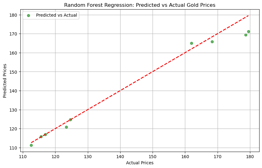
Random Forest Regression - MSE: 20.038521527221764, R²: 0.9730209288210895
6.3 Graph (Random Forest Regression)#
plt.figure(figsize=(10, 6))
plt.scatter(y_test_regression, y_pred_rf, alpha=0.6, color='green', label='Predicted vs Actual')
plt.plot([y_test_regression.min(), y_test_regression.max()], [y_test_regression.min(), y_test_regression.max()], 'r--', linewidth=2)
plt.title('Random Forest Regression: Predicted vs Actual Gold Prices')
plt.xlabel('Actual Prices')
plt.ylabel('Predicted Prices')
plt.legend()
plt.grid(True)
plt.show()
Result#
This graph suggests that the Random Forest Regression model is highly accurate in capturing the relationship between the features and gold prices, making it a reliable choice for price prediction tasks.
7. Linear Regression#
Finally, I applied a Linear Regression model to predict gold prices. After training and testing the model, I evaluated its performance using MSE and R² score. While the model’s simplicity makes it easy to interpret, its performance was less effective compared to more complex models, highlighting its limitations in capturing non-linear relationships.
7.1 Model Training and Prediction (Linear Regression)#
# Linear Regression Model
linear_reg = LinearRegression()
linear_reg.fit(X_train_scaled, y_train_regression)

# Predict on the test set
y_pred_linear = linear_reg.predict(X_test_scaled)
7.2 Evaluation of Linear Regression#
# Evaluate the model
linear_mse = mean_squared_error(y_test_regression, y_pred_linear)
linear_r2 = r2_score(y_test_regression, y_pred_linear)
print(f"Linear Regression - MSE: {linear_mse}, R²: {linear_r2}")
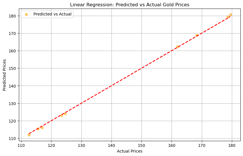
Linear Regression - MSE: 0.4175571796371035, R²: 0.9994378175627683
7.3 Graph#
# Visualization
plt.figure(figsize=(10, 6))
plt.scatter(y_test_regression, y_pred_linear, alpha=0.6, color='orange', label='Predicted vs Actual')
plt.plot([y_test_regression.min(), y_test_regression.max()], [y_test_regression.min(), y_test_regression.max()], 'r--', linewidth=2)
plt.title('Linear Regression: Predicted vs Actual Gold Prices')
plt.xlabel('Actual Prices')
plt.ylabel('Predicted Prices')
plt.legend()
plt.grid(True)
plt.show()
Result#
This graph indicates that the Linear Regression model struggles to accurately capture the relationship between the features and gold prices. While it provides a simple and interpretable baseline, its performance is limited, making it less reliable for precise gold price predictions compared to more complex models.
8. Summary#
Linear Regression and Ridge Regression have nearly perfect alignments between the predicted and actual values along the ideal fit line. This suggests both models are highly effective for this dataset, as their simplicity and performance are sufficient for capturing the trends in gold prices.
Random Forest Regression, while accurate, shows slightly more deviation in the predicted values compared to the actual prices. Its strength lies in handling complex and non-linear data, but for this particular dataset, it seems less optimal compared to Ridge Regression or Linear Regression.
9. Reference#
The dataset is downloaded from https://www.kaggle.com/datasets/franciscogcc/financial-data?resource=download