Linear Regression#
Problem#
Given the training dataset \(x_i\in\mathbb{R}\), \(y_i\in\mathbb{R}\), \(i= 1,2,..., N\), we want to find the linear function
that fits the relations between \(x_i\) and \(y_i\). So that given any \(x\), we can make the prediction
Loss Function and Optimization#
With the training dataset, define the loss function \(L(w,b)\) of parameter \(w\) and \(b\), which is also called mean squared error (MSE)
where \(\hat{y}^{(i)}\) denotes the predicted value of y at \(x_i\), i.e. \(\hat{y}^{(i)} = wx_i+b\).
Our goal is to find the optimal \(w\) and \(b\) that minimize the loss function \(L(w,b)\), i.e.
This is a function of \(w\) and \(b\), and we can analytically solve \(\partial_{w}L = \partial_{b}L =0\), and yields
where \(\bar{X}\) and \(\bar{Y}\) are the mean of \(x\) and of \(y\), and \(\text{Cov}(X,Y)\) denotes the estimated covariance (or called sample covariance) between \(X\) and \(Y\), \(\text{Var}(Y)\) denotes the sample variance of \(Y\).
Evaluating the model#
MSE: The smaller MSE indicates better performance.
MSE depends on the unit. For example, if we replace y[m] by y[mm], than MSE will be \(1000^2\) times the original MSE.
\(R^{2}\) (coefficient of determination): The larger \(R^{2}\) (closer to 1) indicates better performance. Compared with MSE, R-squared is dimensionless, not dependent on the units of variable.
Intuitively, MSE is the “unexplained” variance, and \(R^{2}\) is the proportion of the variance that is explained by the model: If our model is perfect, then MSE is 0, and \(R^{2}\) is 1. If we are using a constant model, then our best prediction is the mean of \(y\), and MSE is the variance of \(y\), and \(R^{2}\) is 0;
import numpy as np
import matplotlib.pyplot as plt

class myLinearRegression:
    '''
    The single-variable linear regression estimator.
    This serves as an example of the regression models from sklearn, with methods fit, predict, and score.
    '''
    def __init__(self):
        '''
        '''
        self.w = None
        self.b = None

    def fit(self, x, y):
        # covariance matrix,
        # bias = True makes the factor 1/N, otherwise 1/(N-1)
        # but it doesn't matter here, since the factor will be cancelled out in the calculation of w

        cov_mat = np.cov(x, y, bias=True)
        # cov_mat[0, 1] is the covariance of x and y, and cov_mat[0, 0] is the variance of x

        self.w = cov_mat[0, 1] / cov_mat[0, 0]
        self.b = np.mean(y) - self.w * np.mean(x)

        # :.3f means 3 decimal places
        print(f'w = {self.w:.3f}, b = {self.b:.3f}')

    def predict(self, x):
        '''
        Predict the output values for the input value x, based on trained parameters

        '''
        ypred = self.w * x + self.b
        return ypred

    def score(self, x, y):
        '''
        Calculate the R^2 score of the model
        '''
        mse =  np.mean((y - self.predict(x))**2)
        var = np.mean((y - np.mean(y))**2)
        Rsquare = 1 - mse / var
        return Rsquare
# Generate synthetic data

np.random.seed(0) # for reproducibility

a = 0
b = 2
N = 20

x = np.random.uniform(a,b,N)
y = 2 * x + 1 + np.random.randn(N)
y_gt = 2 * x + 1

# Fit the model
lm = myLinearRegression()
lm.fit(x, y)
score = lm.score(x, y)


# plot data
plt.plot(x, y, 'o', label='data')
# plot ground truth
plt.plot(x, y_gt, label='ground truth')


# plot the linear regression model
xs = np.linspace(a, b, 100)
plt.plot(xs, lm.predict(xs), label=f'pred, $R^2$={score:.3f}')
plt.legend()

print(f'score = {score:.3f}')
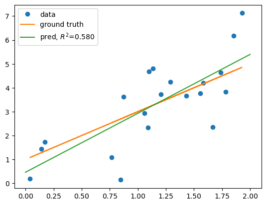
w = 2.467, b = 0.462
score = 0.580

We can also use LinearRegression from sklearn.linear_model to fit the linear model.
# Use the following command to install scikit-learn
# %conda install scikit-learn
# or
# %pip install scikit-learn
from sklearn.linear_model import LinearRegression

reg = LinearRegression()

# x need to be n-sample by p features
reg.fit(x.reshape(-1, 1), y)
print(f'w = {reg.coef_[0]:.3f}, b = {reg.intercept_:.3f}')

score = reg.score(x.reshape(-1, 1), y)
print(f'score = {score:.3f}')
w = 2.467, b = 0.462
score = 0.580
What is the effect of centering the data?#
When \(X\) is centered, the slope \(w\) remains the same, but the intercept \(b\) changes.
The intercept now means the predicted Y when X is at the mean.
x_center = x - np.mean(x)

reg.fit(x_center.reshape(-1, 1), y)
print(f'w = {reg.coef_[0]:.3f}, b = {reg.intercept_:.3f}')
w = 2.467, b = 3.332
When Y is centered, then the intercept \(b\) is 0, and the slope \(w\) is the correlation between \(X\) and \(Y\).
y_center = y - np.mean(y)
reg.fit(x_center.reshape(-1, 1), y_center)
print(f'w = {reg.coef_[0]:.3f}, b = {reg.intercept_:.3f}')
w = 2.467, b = 0.000
What is the effect of scaling the data?#
When \(X/c\) is used, the optimal slope is now \(c w\), and the intercept does not change
# suppose we want to scale x to [0, 1]
scale_factor = np.max(x)
x_scale = x / scale_factor
reg.fit(x_scale.reshape(-1, 1), y)
print(f'w = {reg.coef_[0]:.3f}, b = {reg.intercept_:.3f}')
w = 4.756, b = 0.462
For linear regression, centering and scaling the data (both training and testing data ) does not affect the performance of the model.
For some other models, centering and scaling can be essential
Appendix#
Detailed Derivation of the Optimal Parameters (Not exam material).
The loss function for simple linear regression is given by:
To find the optimal ( w ), we set the partial derivative of ( L ) with respect to ( w ) to zero:
Differentiate with respect to ( w ):
Rearrange this equation to get:
Derivative with respect to \(b\):
This simplifies to:
Or, equivalently:
Substitute \(b\) back into the equation (*), we get:
Expanding this:
Rearranging terms
Now, solving for \(w\):
Recall that \(Cov(X,Y) = E[XY]-E[X]E[Y]\), and \(Var(X) = E[X^2] - E[X]^2\). Divide both the numerator and the denominator by \(N\). We can rewrite the above equation in terms of covariance and variance: $\(w = \frac{Cov(X,Y)}{Var(X)}\)$
This is the final expression for \(w^*\) in simple linear regression, representing the slope of the best-fit line.