Probability and Statistics#
These concepts are important in data science, enabling us to quantify uncertainty and variability in data.
Note: probability and statistics is not a prerequisite for this course. This notebook focuses on the intuitive understanding of these concepts using examples.
Random Experiments#
Example: roll a die is a random experiment. The set of all possible outcomes is the sample space, in this case, \(\{1, 2, 3, 4, 5, 6\}\). An event is a subset of the sample space, e.g., the event “rolling an even number” is \(\{2, 4, 6\}\).
Probability#
There are the following rules for probability:
The probability of any event is between 0 and 1.
The probability of the whole sample space is 1, that is, something in the sample space must happen.
If two events cannot happen at the same time, then the probability of either event happening is the sum of the probabilities of each event.
Example: If we roll a die, the probability of getting k is some positive number between 0 and 1 for each k in \(\{1, 2, 3, 4, 5, 6\}\).
The probability of getting any number between 1 and 6 is 1 (the die cannot land on the edge)
The probability of getting “either 1 or 2” is the probability of getting 1 plus the probability of getting 2.
How to define probability?
This is actually a very interesting question. For our purposes, we will just keep it intuitive.
We say that that the probability of tossing a coin and getting a head is 0.5, because (1) we did it many times and half of the times we got heads, or (2) we believe that the coin is fair and the two outcomes are equally likely.
Random Variables#
Random variables maps each outcome of a random experiment to a number.
Example: If we flip a coin, we can define a random variable \(X\) that is 1 if the coin lands heads, and 0 if the coin lands tails. Here, \(X \in \{0, 1\}\). Alternatively, if we are betting 1 dollar on heads we can define a random variable \(X\) that represent the payoff, \(X \in \{-1, 1\}\).
Discrete Random Variables#
A random variable is discrete if it takes on a finite number of values.
Example: If \(X\) represents the outcome of rolling a die, then \(X \in \{1, 2, 3, 4, 5, 6\}\), with \(P(X = x) = \frac{1}{6}\) for each \(x \in \{1, 2, 3, 4, 5, 6\}\).
Note: usually, X denotes a random variable, while x denotes a specific value of that variable.
Note: we usually consider finite number of outcomes. But there could be infinite but countable number of outcomes. For example, the number of flips until the first head. It could be 1, 2, 3, 4, …, 100, … and so on (if we are unlucky).
Continuous Random Variables#
A random variable is continuous if it can take on any value in an interval.
Example: If \(Y\) denotes the time (in minutes) for the next bus to arrive, then \(Y \in [0, \infty)\). Here, \(Y\) could be 2.5 minutes, 3.14159 minutes, or any other positive real number.
Distributions#
The probability distribution of a random variable provides a complete description of the likelihood of various outcomes.
probability mass function (PMF)#
For a discrete variable \(X\), the PMF is the function \(p(x) = P(X = x)\) that gives the probability that \(X\) is equal to a particular value \(x\).
Example: If \(X\) represents the outcome of rolling a die, then we have the PMF \(p(x) = \frac{1}{6}\) for each \(x \in \{1, 2, 3, 4, 5, 6\}\), and 0 otherwise.
Note that \(\sum_{\text{all outcome x}} p(x) = 1\).
probability density function (PDF)#
For a continuous variable \(Y\), the PDF, \(f(y)\), is such that the probability of \(Y\) falling in an interval \([a, b]\) is given by the integral of \(f(y)\) over that interval:
Example: If \(Y\) is uniformly distributed on \([0, 1]\), then \(f(y) = 1\) for \(y \in [0, 1]\), and 0 otherwise.
Note that \(\int_{-\infty}^{\infty} f(y) dy = 1\).
What is the relationship between random variables and data?#
Data are realizations of random variables. We collect data to learn about the underlying random process.
For example: let’s say we want to know if a coin is fair – this is a question about the underlying random process, the distribution of the random variable. To answer this question, we start flipping the coin and recording the outcomes. This is the data, which is the realization of the random variable.
How to estimate probabilities?#
We can estimate the probability of an event by looking at the relative frequency of that event:
Expectation#
The expectation or expected value of a random variable the average value of the random variable, weighted by the probability of each value. You can always think of a random variable as the “payoff” in a game, and the expectation is the “average payoff” in each round of the game if you play it many times.
For a discrete random variable \(X\), \(E[X] = \sum_{x} x \cdot P(X = x)\).
Example: If \(X\) represents the outcome of rolling a die, then \(E[X] = \sum_{x=1}^{6} x \cdot \frac{1}{6} = 3.5\).
For a continuous random variable \(Y\), \(E[Y] = \int_{-\infty}^{\infty} y \cdot f_Y(y) \, dy\).
Example: If \(Y\) is uniformly distributed on \([0, 1]\), then \(E[Y] = \int_{0}^{1} y \cdot 1 \, dy = \frac{1}{2}\).
We have \(E[aX + bY] = aE[X] + bE[Y]\) for any constants \(a\) and \(b\).
How to estimate the expectation of a random variable from data?#
One common approach is to use the sample mean: if \(X_1, X_2, \ldots, X_n\) are independent and identically distributed (i.i.d.) samples of \(X\), then the sample mean \(\bar{X} = \frac{1}{n} \sum_{i=1}^{n} X_i\) is an estimator of \(E[X]\)
Variance#
Variance quantifies the spread of a distribution around its mean, reflecting the variability of the random variable. \(\text{Var}(X) = E[(X - E[X])^2]\)
We have \(\text{Var}(aX+b) = a^2 \text{Var}(X)\) for any constant \(a\) and \(b\).
How to estimate the variance of a random variable from data?#
One common approach is to use the sample variance: if \(X_1, X_2, \ldots, X_n\) are i.i.d. samples of \(X\). Let \(\bar{X}\) be the sample mean, then the sample variance \(S^2 = \frac{1}{n} \sum_{i=1}^{n} (X_i - \bar{X})^2\) is an estimator of \(\text{Var}(X)\).
Note: you might see 1/(n-1) instead of 1/n in the definition of sample variance. For large n, the difference is negligible.
Standard Deviation#
The standard deviation is the square root of the variance, \(\sigma^2 = \text{Var}(X)\), providing a measure of the spread of a distribution in the same units as the random variable.
Covariance#
Covariance provides a measure of how two random variables change together. For example, if we treat weight and height as random variables, then knowing that someone is taller than average might make it more likely that they have above-average weight.
For random variables \(X\) and \(Y\), the covariance is defined as \(\text{Cov}(X, Y) = E[(X - E[X])(Y - E[Y])]\).
Correlation#
Correlation is a standardized measure of how two random variables change together, ranging from -1 to 1. \( \text{Corr}(X, Y) = \frac{\text{Cov}(X, Y)}{\sqrt{\text{Var}(X) \cdot \text{Var}(Y)}}\).
Causality#
Correlation is Not Causation#
Correlation measures the strength and direction of a linear relationship between two variables. However, it does not imply causation.
For example: Ice cream sales and drowning incidents might be correlated (both increase in the summer), but one does not cause the other.
See Spurious Correlations for more examples.
Independent is Not “No-Causation”#
Suppose two light switches, A and B, control the light bulb in the following way: the light is on if (1) A on B off or (2) A off B on. Assume the switch are independent “coin flips”: equally likely to be on or off. Then knowing the state of switch A gives no information about the light. But there is still a “cause and effect” relationship between the switch and the light. We only see this relationship when we consider both switches together. (Example adapted from here)
Establishing Causality#
Establishing causality is challenging, and might require controlled experiments beyond observational data.
Computation#
The following Python code demonstrates how to do computation related to the previous concepts.
Estimating probabilities#
When we don’t know the probability of some event, we can estimate it by running the experiment many times and calculating the relative frequency of the event.
# generate list of random integers
import numpy as np


# estimating the probability of rolling a 6
# n is number of experiments, or sample size
# larger n, "closer" to true probability
n = 100
x = np.random.randint(1, 7, n)
p = np.sum(x == 6) / 100
print(p)
0.15
# uniform distribution on [0, 1]
# estimating the probability hitting [0, 0.5]
n = 100
x = np.random.rand(n)
p = np.sum(x < 0.5) / n
print(p)
0.53
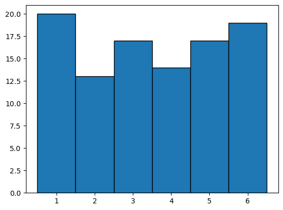
visualizing distribution using histogram#
# to install seaborn
# %conda install seaborn
# %pip install numpy
# %conda install numpy
# for to visualize the distribution, we can use a histogram
import matplotlib.pyplot as plt

n = 100
x = np.random.randint(1, 7, n)

plt.hist(x, bins=6, range=(0.5, 6.5),edgecolor='black')
(array([20., 13., 17., 14., 17., 19.]),
 array([0.5, 1.5, 2.5, 3.5, 4.5, 5.5, 6.5]),
 <BarContainer object of 6 artists>)
# can also use seaborn
# import seaborn
# seaborn.histplot(x, discrete=True)
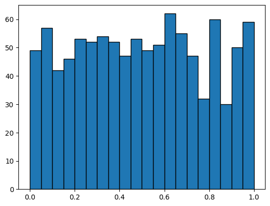
# generate uniform random numbers
x = np.random.rand(1000)
# seaborn.histplot(x, stat='density')
plt.hist(x, bins=20, range=(0, 1), edgecolor='black')
(array([49., 57., 42., 46., 53., 52., 54., 52., 47., 53., 49., 51., 62.,
        55., 47., 32., 60., 30., 50., 59.]),
 array([0.  , 0.05, 0.1 , 0.15, 0.2 , 0.25, 0.3 , 0.35, 0.4 , 0.45, 0.5 ,
        0.55, 0.6 , 0.65, 0.7 , 0.75, 0.8 , 0.85, 0.9 , 0.95, 1.  ]),
 <BarContainer object of 20 artists>)
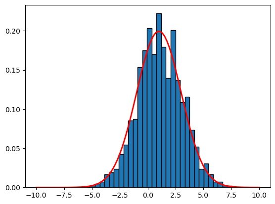
# gaussian normal distribution
# as n increases, the histogram looks more like the density function
# mu is the mean, sigma is the standard deviation
mu = 1
sigma = 2
n = 1000 # sample size
x  = np.random.normal(mu, sigma, n) # generate samples from the normal distribution

# plot the histogram
plt.hist(x, bins=30, edgecolor='black', density=True)


# plot the density function
x = np.linspace(-10, 10, 100)
f = (1/(sigma * np.sqrt(2 * np.pi)) *
     np.exp(- (x - mu)**2 / (2 * sigma**2)))
plt.plot(x,f,linewidth=2, color='r')
[<matplotlib.lines.Line2D at 0x11bc71a90>]
How to estimate the E[X]#
the expecttion can be estimated by the sample mean
Let \(X_1, X_2, \ldots, X_n\) be samples from a random variable \(X\). The sample mean \(\bar{X} = \frac{1}{n} \sum_{i=1}^n X_i\) approximate the \(E[X]\)
Law of large numbers#
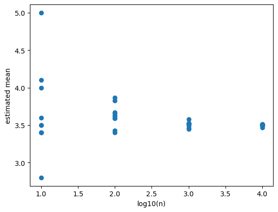
The law of large numbers states that the sample mean converges to the expected value as the sample size increases.
# In each experiment, we draw n samples and estimate the mean.
# For small n, each estimation might have large variability for different repetitions.
# As n increases, the variability decreases.
# For very large n, the estimates are almost the same as the true mean and the variability is very small.

# use n sample to estimate the mean
n = [10,100,1000,10000]

# number of repetitions for each n
k = 10

# store the estimates, each row is a different n, each column is a different repetition
estiamtes = np.zeros((len(n), k))

# sample sizes
logn = [] # log10 of n
means = [] # estimated mean

for ni in n:
    for k in range(10):
        x = np.random.randint(1, 7, ni)
        logn.append(np.log10(ni))
        means.append(np.mean(x))

fig, ax = plt.subplots()
# scatter plot of
ax.scatter(logn, means)
ax.set_xlabel('log10(n)')
ax.set_ylabel('estimated mean')
Text(0, 0.5, 'estimated mean')
Estimation of variance#
# estimate variance of dice row
n = 100
x = np.random.randint(1, 7, n)
var1 = np.var(x)
var2 = np.mean((x - x.mean())**2)
print(var1, var2)
3.1291000000000007 3.1291000000000007
Computing covariance#
np.cov(x, y) return a 2x2 matrix M, where M[0, 0] is the variance of x, M[1, 1] is the variance of y, M[0, 1] is the covariance of x and y, and M[1, 0] is the covariance of y and x, which is the same as M[0, 1]. Similarly, np.corrcoef(x, y) returns the correlation matrix.
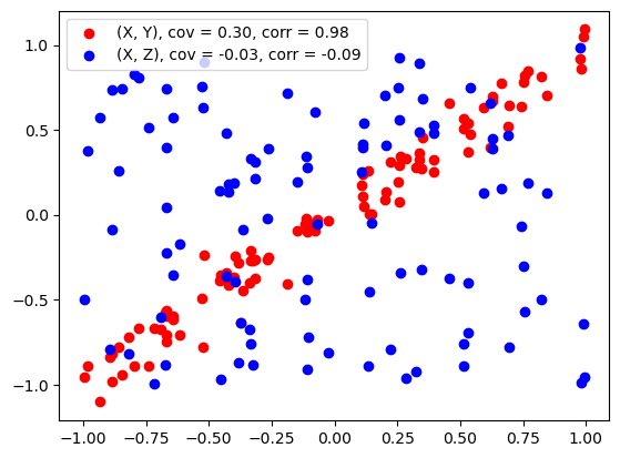
Visualizing correlation#
from matplotlib import pyplot as plt
import numpy as np

n = 100 # sample size

# X is a random variable uniformly distributed on [0, 1]
x = np.random.uniform(-1, 1, n)

# Y is a linear function of X plus noise
y = x + np.random.normal(0, 0.1, n)

# z is independent of X
z = np.random.uniform(-1, 1, n)

cov_xy = np.cov(x, y)[0, 1]
cov_xz = np.cov(x, z)[0, 1]

corr_xy = np.corrcoef(x, y)[0, 1]
corr_xz = np.corrcoef(x, z)[0, 1]

# scatter plot
fig, ax = plt.subplots()
# plot x vs y and x vs z, different colors, show name
ax.scatter(x, y, color='red', label='(X, Y), cov = %.2f, corr = %.2f' % (cov_xy, corr_xy))
ax.scatter(x, z, color='blue', label='(X, Z), cov = %.2f, corr = %.2f' % (cov_xz, corr_xz))
# show legend
ax.legend()
plt.show()
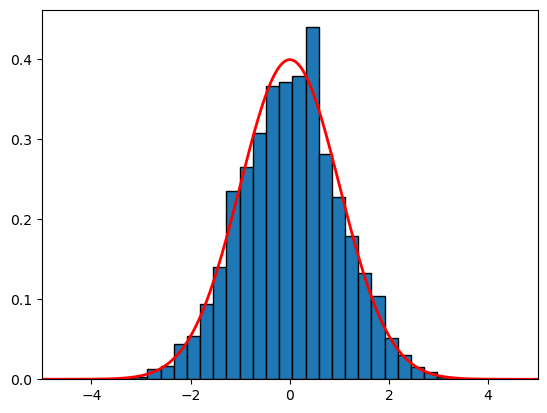
Central limit theorem#
Roughly speaking, sample average are normally distributed for large sample sizes, regardless of the distribution of the underlying random variable!
This explains why the normal distribution is so common.
If \(X_1, X_2, \ldots, X_n\) are independent and identically distributed random variables with mean \(\mu\) and variance \(\sigma^2\), if we define
then for large n, Z is approximately normally distributed with mean 0 and variance 1.
# we know that the coin flip has a mean of 0.5 and a variance of 0.25
gaussian_density = lambda x,mu,sigma: (1/(sigma * np.sqrt(2 * np.pi)) * np.exp(- (x - mu)**2 / (2 * sigma**2)))

mu = 0.5
sigma = np.sqrt(0.25)

# number of experiments, in each experiment we draw n samples, and estimate the mean
N = 10000
n = 1000

z_samples = []


for i in range(N):

	# draw n samples
	x = np.random.randint(0, 2, n)
	# compute the sample mean
	sample_mean = np.mean(x)

	# do the transformation
	z = np.sqrt(n)*(sample_mean -  mu)/sigma

	z_samples.append(z)

# plot the histogram of z_samples
plt.hist(z_samples, bins=30, edgecolor='black', density=True)


# overlay the density function of the standard normal distribution
x = np.linspace(-10, 10, 1000)
y = gaussian_density(x, 0, 1)
plt.plot(x,y,linewidth=2, color='r')
plt.xlim(-5,5)
(-5.0, 5.0)
