Title: Should I investing to SIRI stock ? Reason?#
Author: Nguyen Bui
Course Project, UC Irvine, Math 10, Fall 24
I would like to post my notebook on the course’s website.
Section 1: Itroduction#
My project aims to take advantage of Python’s powerful data analysis and machine learning capabilities to assess the investment potential of SIRI stock and predict the future of the stock. By delving into historical stock price dataset, financial metrics, and industry trends, we seek to uncover valuable insights that can inform investment strategies.We can see if the new trend happening and able to entry the buy position early to make money on the market.
Section 2: Load The Dataset#
Important Just let the Viewer of my project know that the price in the dataset below got divied by 10 mean that 2 = 20.
This is the stock price data for SIRIUS XM Holdings Inc. from 09/13/1994 to 06/21/2024. The column included:raded
*Date: The date of the stock price
*Open: The opening price of the stock
*High: The highest price of the stock
*Low: The lowest price of the stock
*Close: The closing price of the stock
*Volume: The volume of stocks traded
*Adjclose: The adjusted closing price amends a stock’s closing price to reflect that stock’s value after accounting for any corporate actions
*Ticker: Symbol of company stock
Load The Dataset#
import pandas as pd

file_path = "SIRI_stock_data.csv"
try:
    siri_stock_data = pd.read_csv(file_path)
    print("Data loaded successfully!")
    print(siri_stock_data)
except FileNotFoundError:
    print(f"Error: The file '{file_path}' was not found.")
except Exception as e:
    print(f"An error occurred: {e}")
Data loaded successfully!
      Unnamed: 0   open      high    low     close  adjclose    volume ticker
0     1994-09-13  4.500  4.875000  4.500  4.625000  4.015482     74000   SIRI
1     1994-09-14  4.500  4.750000  3.625  4.375000  3.798428    335100   SIRI
2     1994-09-15  4.500  4.546875  4.375  4.546875  3.947653     43600   SIRI
3     1994-09-16  4.375  4.750000  4.250  4.750000  4.124009    171900   SIRI
4     1994-09-19  4.875  4.875000  4.875  4.875000  4.232535      2100   SIRI
...          ...    ...       ...    ...       ...       ...       ...    ...
7491  2024-06-14  2.510  2.630000  2.490  2.610000  2.610000  75254700   SIRI
7492  2024-06-17  2.630  2.670000  2.550  2.650000  2.650000  45854400   SIRI
7493  2024-06-18  2.660  2.770000  2.650  2.770000  2.770000  64476800   SIRI
7494  2024-06-20  2.840  2.940000  2.760  2.900000  2.900000  38796600   SIRI
7495  2024-06-21  2.955  3.030000  2.950  2.995000  2.995000  47781660   SIRI

[7496 rows x 8 columns]
The dataset is a long period of time, then I will reduce it to 6 months Dataset.#
import pandas as pd
file_path = "SIRI_stock_data.csv"
siri_stock_data = pd.read_csv(file_path)
siri_stock_data['Unnamed: 0'] = pd.to_datetime(siri_stock_data['Unnamed: 0'])
start_date = '2024-01-01'
end_date = '2024-06-21'
filtered_data = siri_stock_data[(siri_stock_data['Unnamed: 0'] >= start_date) & (siri_stock_data['Unnamed: 0'] <= end_date)]
print(filtered_data)
filtered_data.to_csv('SIRI_stock_data_filtered.csv', index=False)
     Unnamed: 0   open  high   low  close  adjclose    volume ticker
7377 2024-01-02  5.450  5.68  5.42  5.490  5.460763  15594800   SIRI
7378 2024-01-03  5.490  5.52  5.37  5.440  5.411030  14631900   SIRI
7379 2024-01-04  5.400  5.47  5.29  5.430  5.401083   8881700   SIRI
7380 2024-01-05  5.410  5.55  5.37  5.460  5.430923  15562600   SIRI
7381 2024-01-08  5.450  5.55  5.42  5.480  5.450817  13423800   SIRI
...         ...    ...   ...   ...    ...       ...       ...    ...
7491 2024-06-14  2.510  2.63  2.49  2.610  2.610000  75254700   SIRI
7492 2024-06-17  2.630  2.67  2.55  2.650  2.650000  45854400   SIRI
7493 2024-06-18  2.660  2.77  2.65  2.770  2.770000  64476800   SIRI
7494 2024-06-20  2.840  2.94  2.76  2.900  2.900000  38796600   SIRI
7495 2024-06-21  2.955  3.03  2.95  2.995  2.995000  47781660   SIRI

[119 rows x 8 columns]
The mean, standard deviation, minimum, and maximum of the closing price of the stock#
a) Compute statistical measures for the ‘close’ column#
mean_close = filtered_data['close'].mean()
std_close = filtered_data['close'].std()
min_close = filtered_data['close'].min()
max_close = filtered_data['close'].max()
b) Results of closing Price#
# Print the results
print(f"Mean of Closing Price: {mean_close:.2f}")
print(f"Standard Deviation of Closing Price: {std_close:.2f}")
print(f"Minimum Closing Price: {min_close:.2f}")
print(f"Maximum Closing Price: {max_close:.2f}")
Mean of Closing Price: 3.91
Standard Deviation of Closing Price: 0.99
Minimum Closing Price: 2.53
Maximum Closing Price: 5.49
The Date of the highest stock price (“High”) occurred, and the opening and closing prices for that day of the stock:#
a) Find the row with the highest stock price (‘High’)#
max_high_row = filtered_data.loc[filtered_data['high'].idxmax()]
b) Extract relevant information and print the results#
highest_price_date = max_high_row['Unnamed: 0']
highest_price_open = max_high_row['open']
highest_price_close = max_high_row['close']

print(f"Date of Highest Stock Price: {highest_price_date}")
print(f"Opening Price on that day: {highest_price_open:.2f}")
print(f"Closing Price on that day: {highest_price_close:.2f}")
Date of Highest Stock Price: 2024-01-02 00:00:00
Opening Price on that day: 5.45
Closing Price on that day: 5.49
The Graph for the High price and Low Price in that period of Time:#
a) Plot the ‘High’ and ‘Low’ prices#
import matplotlib.pyplot as plt
plt.figure(figsize=(12, 6))
plt.plot(filtered_data['Unnamed: 0'], filtered_data['high'], label='High Price', color='green', linewidth=1.5)
plt.plot(filtered_data['Unnamed: 0'], filtered_data['low'], label='Low Price', color='red', linewidth=1.5)
plt.title('High and Low Prices Over Time', fontsize=16)
plt.xlabel('Date', fontsize=12)
plt.ylabel('Price', fontsize=12)
plt.legend(fontsize=12)
plt.grid(True)
plt.tight_layout()
plt.xticks(rotation=45)
plt.show()
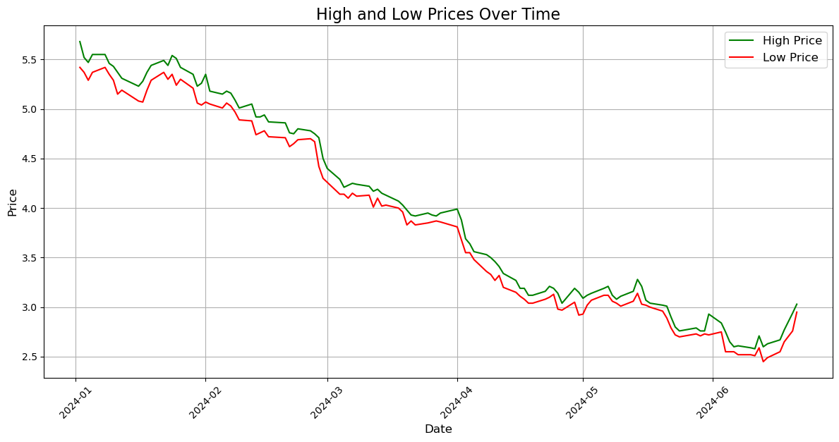
Note: The gap between the High and low price mean that the price of the stock moving only between the gap and can not pass the gap. From there you can predict the range of the SIRI Stock price the next day.
Section 3 : Moving Average for Close’ price of the stock SIRI and the 7-day moving average of the ‘Close’ price#
Calculate the 7-day moving average of the ‘Close’ price#
import matplotlib.pyplot as plt
filtered_data['7-day Moving Average'] = filtered_data['close'].rolling(window=7).mean()
/tmp/ipykernel_146/474738594.py:2: SettingWithCopyWarning:
A value is trying to be set on a copy of a slice from a DataFrame.
Try using .loc[row_indexer,col_indexer] = value instead

See the caveats in the documentation: https://pandas.pydata.org/pandas-docs/stable/user_guide/indexing.html#returning-a-view-versus-a-copy
  filtered_data['7-day Moving Average'] = filtered_data['close'].rolling(window=7).mean()
Plot the ‘Close’ price and the 7-day moving average#
# Plot the 'Close' price and the 7-day moving average
plt.figure(figsize=(12, 6))
plt.plot(filtered_data['Unnamed: 0'], filtered_data['close'], label='Close Price', color='blue', linewidth=1.5)
plt.plot(filtered_data['Unnamed: 0'], filtered_data['7-day Moving Average'], label='7-Day Moving Average', color='orange', linewidth=2)

# Add labels, title, and legend
plt.title('Close Price and 7-Day Moving Average', fontsize=16)
plt.xlabel('Date', fontsize=12)
plt.ylabel('Price', fontsize=12)
plt.legend(fontsize=12)
plt.grid(True)
plt.tight_layout()

# Rotate the x-axis labels for better readability
plt.xticks(rotation=45)

# Display the plot
plt.show()
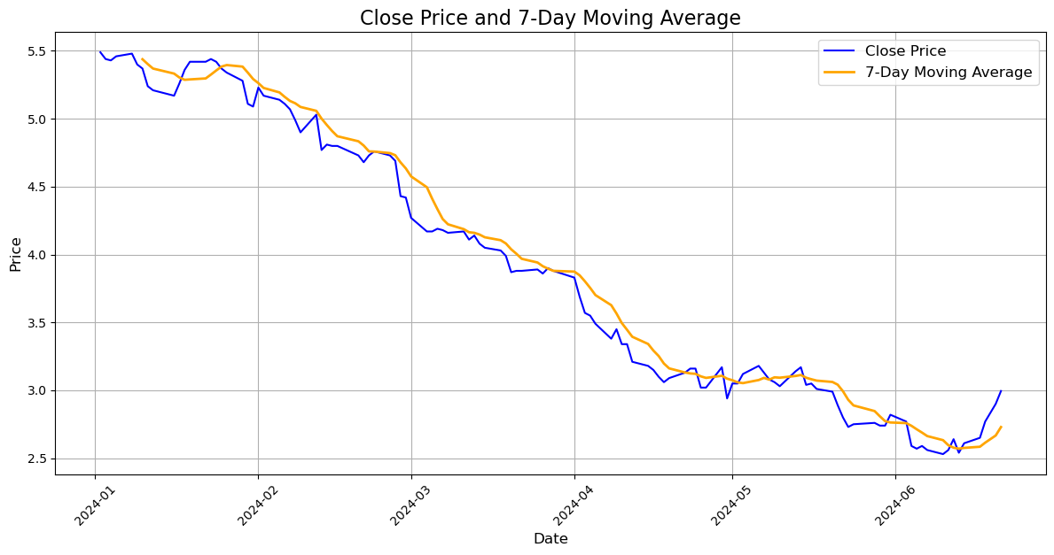
Note: Based on the Data graph above I can understand that from January 2024 to June 2024 the stock price has an obvious downward trend, and also I see the close price somewhat always under the 7-day moving average. However, since pass June 2024, the close price has already been above the 7-day Moving Average. Since then, I predict the stock will begin starting a trend. It is an important factor why I invest in Sirius XM Holdings Inc.( Let me confirm again this is only based on my perspective and my opinion).
Section 4: Linear Regression#
MSE and R-squared prediction :#
import pandas as pd
import numpy as np
from sklearn.model_selection import train_test_split
from sklearn.linear_model import LinearRegression
from sklearn.metrics import mean_squared_error, r2_score
import matplotlib.pyplot as plt
filtered_data['Unnamed: 0'] = pd.to_datetime(filtered_data['Unnamed: 0'])
filtered_data['Date_Num'] = (filtered_data['Unnamed: 0'] - filtered_data['Unnamed: 0'].min()).dt.days
/tmp/ipykernel_146/1722334898.py:7: SettingWithCopyWarning:
A value is trying to be set on a copy of a slice from a DataFrame.
Try using .loc[row_indexer,col_indexer] = value instead

See the caveats in the documentation: https://pandas.pydata.org/pandas-docs/stable/user_guide/indexing.html#returning-a-view-versus-a-copy
  filtered_data['Unnamed: 0'] = pd.to_datetime(filtered_data['Unnamed: 0'])
/tmp/ipykernel_146/1722334898.py:8: SettingWithCopyWarning:
A value is trying to be set on a copy of a slice from a DataFrame.
Try using .loc[row_indexer,col_indexer] = value instead

See the caveats in the documentation: https://pandas.pydata.org/pandas-docs/stable/user_guide/indexing.html#returning-a-view-versus-a-copy
  filtered_data['Date_Num'] = (filtered_data['Unnamed: 0'] - filtered_data['Unnamed: 0'].min()).dt.days
a) Define features (X) and target variable (y)#
X = filtered_data[['Date_Num']]
y = filtered_data['close']
b) Split the data into training and testing sets#
X_train, X_test, y_train, y_test = train_test_split(X, y, test_size=0.2, random_state=42)

model = LinearRegression()
model.fit(X_train, y_train)
y_pred = model.predict(X_test)
c) Evaluate the model#
mse = mean_squared_error(y_test, y_pred)
r2 = r2_score(y_test, y_pred)

print(f"Mean Squared Error (MSE): {mse:.2f}")
print(f"R-squared (R2): {r2:.2f}")
Mean Squared Error (MSE): 0.04
R-squared (R2): 0.96
Graph of Linear Regression : Date vs. Close Price#
plt.figure(figsize=(12, 6))
plt.scatter(X, y, color='blue', label='Actual Data', alpha=0.6)
plt.plot(X, model.predict(X), color='red', label='Regression Line', linewidth=2)
plt.title('Linear Regression: Date vs. Close Price', fontsize=16)
plt.xlabel('Days Since Start', fontsize=12)
plt.ylabel('Close Price', fontsize=12)
plt.legend(fontsize=12)
plt.grid(True)
plt.tight_layout()
plt.show()
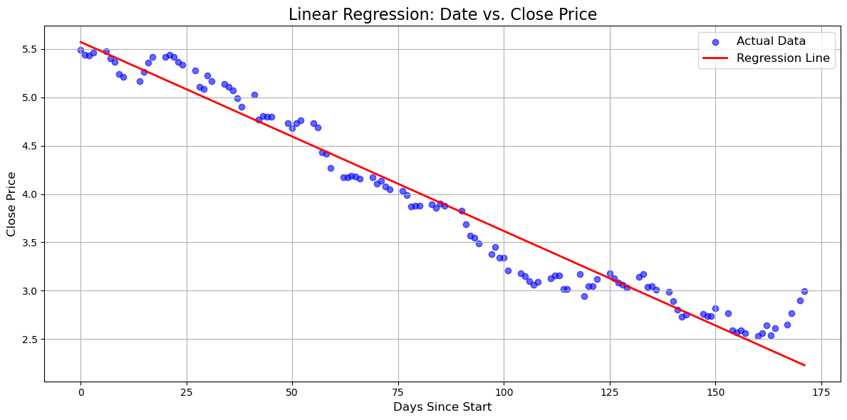
Decreasing Price: The downward slope suggests that the asset’s value has been declining over the observed period. This could be due to various factors like market sentiment, economic conditions, or company-specific news.
Volatility: The scatter of data points around the line indicates some level of volatility in the asset’s price. It doesn’t follow a perfectly linear path, suggesting that other factors might be influencing the price fluctuations.
Section 5: Ridge Regression#
MSE and Rigde Coeffiecnts#
import pandas as pd
from sklearn.model_selection import train_test_split
from sklearn.linear_model import Ridge
from sklearn.metrics import mean_squared_error

file_path = "SIRI_stock_data.csv"
data = pd.read_csv(file_path)
data['Unnamed: 0'] = pd.to_datetime(data['Unnamed: 0'])
start_date = '2024-01-01'
end_date = '2024-06-21'
filtered_data = data[(data['Unnamed: 0'] >= start_date) & (data['Unnamed: 0'] <= end_date)]
X = filtered_data[['open', 'high', 'low', 'volume']]
y = filtered_data['close']
X_train, X_test, y_train, y_test = train_test_split(X, y, test_size=0.2, random_state=42)
ridge = Ridge(alpha=1.0)
ridge.fit(X_train, y_train)
y_pred = ridge.predict(X_test)
mse = mean_squared_error(y_test, y_pred)
print(f"Mean Squared Error: {mse}")
print("Ridge Coefficients:", ridge.coef_)
Mean Squared Error: 0.002026362119631123
Ridge Coefficients: [2.43260057e-01 3.45494567e-01 4.08757455e-01 2.29947433e-10]
/opt/conda/envs/anaconda-2024.02-py310/lib/python3.10/site-packages/sklearn/linear_model/_ridge.py:211: LinAlgWarning: Ill-conditioned matrix (rcond=4.20863e-17): result may not be accurate.
  return linalg.solve(A, Xy, assume_a="pos", overwrite_a=True).T
Graph Ridge Regression: Actual VS Predicted#
# Plotting Actual vs Predicted values
plt.figure(figsize=(10, 6))
plt.scatter(y_test, y_pred, alpha=0.7, color='b', label='Predicted vs Actual')
plt.plot([y_test.min(), y_test.max()], [y_test.min(), y_test.max()], 'r--', lw=2, label='Perfect Prediction')
plt.title("Ridge Regression: Actual vs Predicted")
plt.xlabel("Actual Close Prices")
plt.ylabel("Predicted Close Prices")
plt.legend()
plt.grid(True)
plt.show()
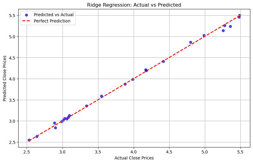
The points closely align with the red dashed line, suggesting that the Ridge Regression model has high predictive accuracy.
Minor deviations from the line imply small prediction errors, but overall, the model performs well.
Both the actual and predicted values are within a range of approximately 2.5 to 5.5, indicating the scale of the target variable.
In conclusion, this graph demonstrates that the Ridge Regression model is effective in predicting the close prices, with predictions closely matching the actual values.
Section 6 : Lasso Regression#
import pandas as pd
from sklearn.model_selection import train_test_split
from sklearn.linear_model import Lasso
from sklearn.metrics import mean_squared_error, r2_score

file_path = "SIRI_stock_data_filtered.csv"
siri_stock_data = pd.read_csv(file_path)

siri_stock_data['Unnamed: 0'] = pd.to_datetime(siri_stock_data['Unnamed: 0'])
siri_stock_data = siri_stock_data.drop(columns=['Unnamed: 0', 'ticker'])

X = siri_stock_data.drop(columns=['close'])
y = siri_stock_data['close']

X_train, X_test, y_train, y_test = train_test_split(X, y, test_size=0.2, random_state=42)

lasso = Lasso(alpha=0.1)
lasso.fit(X_train, y_train)

y_pred = lasso.predict(X_test)

mse = mean_squared_error(y_test, y_pred)
r2 = r2_score(y_test, y_pred)

print("Mean Squared Error:", mse)
print("R-squared:", r2)
print("Lasso Coefficients:", lasso.coef_)
Mean Squared Error: 0.020127919578618255
R-squared: 0.9795766660511636
Lasso Coefficients: [ 0.00000000e+00  8.43969115e-01  0.00000000e+00  0.00000000e+00
 -5.78821947e-09]
Graph For Lasso Regression : Predicted vs Actual#
import matplotlib.pyplot as plt
plt.figure(figsize=(10, 6))
plt.scatter(y_test, y_pred, alpha=0.6, color='blue', label='Predicted vs Actual')
plt.plot([y_test.min(), y_test.max()], [y_test.min(), y_test.max()], color='red', linewidth=2, label='Perfect Fit Line')
plt.xlabel("Actual Close Prices")
plt.ylabel("Predicted Close Prices")
plt.title("Lasso Regression: Predicted vs Actual")
plt.legend()
plt.grid()
plt.show()
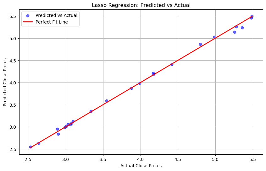
The majority of points seem to be close to the perfect fit line, suggesting that the Lasso Regression model has performed well.
However, any noticeable deviations or patterns in the scatter might indicate areas where the model could improve.
Additional: Volume vs Close Price#
data['Unnamed: 0'] = pd.to_datetime(data['Unnamed: 0'])
start_date = '2024-01-01'
end_date = '2024-06-21'
filtered_data = data[(data['Unnamed: 0'] >= start_date) & (data['Unnamed: 0'] <= end_date)]

plt.figure(figsize=(10, 6))
plt.scatter(filtered_data['volume'], filtered_data['close'], alpha=0.7, color='blue')
plt.title("Volume vs Close Price", fontsize=14)
plt.xlabel("Volume", fontsize=12)
plt.ylabel("Close Price", fontsize=12)
plt.grid(True)
plt.show()
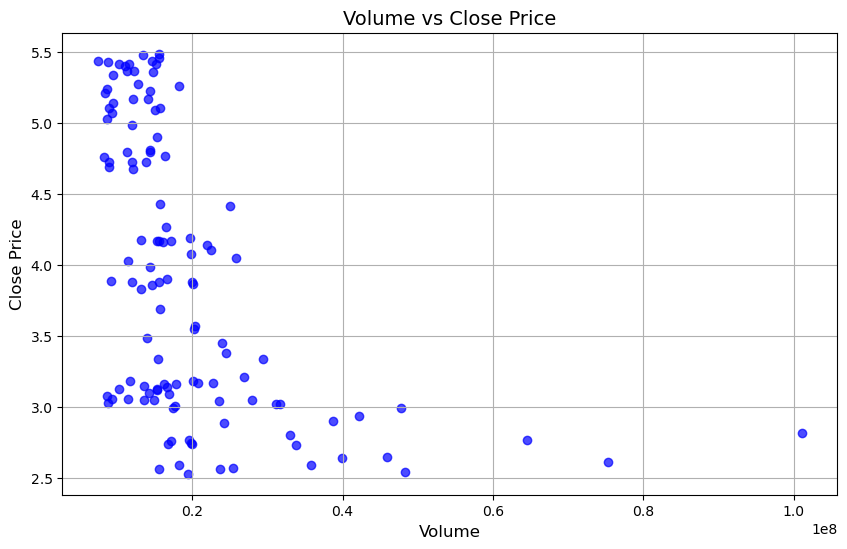
Volume Distribution: Most of the data points are clustered at lower volume values (below 0.2e8). Few points are present at higher volumes.
Close Price Range: The prices range from approximately 2.5 to 5.5.
Relationship: There appears to be a negative trend—higher volumes tend to correlate with lower close prices. Most points with high closing prices are concentrated in low-volume regions.
Also, This graph suggests that stocks with lower trading volumes tend to have higher closing prices, while higher trading volumes might correspond to lower closing prices.
Section 7: K-NN Classification on the Dataset#
import pandas as pd
from sklearn.model_selection import train_test_split
from sklearn.neighbors import KNeighborsClassifier
from sklearn.metrics import accuracy_score, classification_report
import numpy as np

file_path = "SIRI_stock_data.csv"
data = pd.read_csv(file_path)

data['Unnamed: 0'] = pd.to_datetime(data['Unnamed: 0'])
start_date = '2024-01-01'
end_date = '2024-06-21'
filtered_data = data[(data['Unnamed: 0'] >= start_date) & (data['Unnamed: 0'] <= end_date)]

filtered_data['price_movement'] = np.where(filtered_data['close'] > filtered_data['open'], 1, 0)
X = filtered_data[['open', 'high', 'low', 'volume']]
y = filtered_data['price_movement']
X_train, X_test, y_train, y_test = train_test_split(X, y, test_size=0.2, random_state=42)

k = 5
knn = KNeighborsClassifier(n_neighbors=k)
knn.fit(X_train, y_train)

y_pred = knn.predict(X_test)
accuracy = accuracy_score(y_test, y_pred)
print(f"Accuracy: {accuracy:.2f}")
print("\nClassification Report:")
print(classification_report(y_test, y_pred))
Accuracy: 0.58

Classification Report:
              precision    recall  f1-score   support

           0       0.72      0.72      0.72        18
           1       0.17      0.17      0.17         6

    accuracy                           0.58        24
   macro avg       0.44      0.44      0.44        24
weighted avg       0.58      0.58      0.58        24
/tmp/ipykernel_146/4249287838.py:15: SettingWithCopyWarning:
A value is trying to be set on a copy of a slice from a DataFrame.
Try using .loc[row_indexer,col_indexer] = value instead

See the caveats in the documentation: https://pandas.pydata.org/pandas-docs/stable/user_guide/indexing.html#returning-a-view-versus-a-copy
  filtered_data['price_movement'] = np.where(filtered_data['close'] > filtered_data['open'], 1, 0)
Accuracy: 0.58 - This indicates that the model correctly predicted 58% of the instances. While it’s not a perfect score, it’s a decent starting point.
Macro Average: 0.44 - This considers the average performance across both classes. It’s lower than the accuracy, suggesting that the model might have struggled with one of the classes.
Weighted Average: 0.58 - This is similar to accuracy but takes into account the class imbalance. It’s the same as the overall accuracy here, which means the class imbalance didn’t significantly affect the weighted average.
Step 8: In Conclusion,#
By the end of this project, I am gaining a deeper understanding of SIRI’s investment potential. The analysis will provide insights into the company’s financial performance, market sentiment, future prospects, and future trend lines. Additionally, the machine learning model will offer a quantitative approach to predicting stock price movements, aiding in informed decision-making. Through this project helped me to deeply understand that the stock has been undervalued, but the price of the stock is increasing or decreasing due to multiple factors. That is why I analyzed the historical data price, but it is not enough that I have to consider more factors about the Stock company to decide whether to invest in it or not.