Prediction and visualization of various factors affecting Rejection rates in the weaving production

Author:Krishna Saraogi

ID:26635088

Course Project, UC Irvine, Math 10, Fall 24

I would like to post my notebook on the course’s website. Yes

#Introduction

Rejection rates in weaving production are a critical indicator of manufacturing efficiency and product quality. Accurate forecasting and analysis of these rejection rates are highly valuable for manufacturers aiming to minimize waste, optimize resources, and enhance output. Decision-makers in the textile industry, such as production managers and quality control teams, can use these forecasts to implement proactive measures that improve overall productivity.

In this project, I began by compiling and preprocessing a dataset containing various production metrics, such as fabric requirements, beam lengths, and shrinkage allowances. I conducted a series of exploratory data analyses to understand the relationships between these factors and rejection rates. Finally, I applied a range of regression models, including traditional statistical methods and advanced machine learning algorithms, to determine which approach offers the most accurate and actionable predictions for rejection rates.

I have taken the data frame from https://www.kaggle.com/datasets/azminetoushikwasi/textile-weaving-dataset-to-predict-rejection/data

#Importing the necessary liabraries
import numpy as np
import pandas as pd
import matplotlib.pyplot as plt
import seaborn as sns
from sklearn.model_selection import train_test_split,cross_val_score,RandomizedSearchCV
from sklearn.linear_model import LinearRegression
from sklearn.ensemble import RandomForestRegressor,GradientBoostingRegressor
from sklearn.preprocessing import PolynomialFeatures
from sklearn.metrics import mean_squared_error, r2_score
from sklearn.preprocessing import StandardScaler
from sklearn.svm import SVR
from sklearn.tree import export_graphviz, plot_tree
import graphviz
from xgboost import XGBRegressor

#loading and showcasing the first 5 rows of the dataset
dataset = pd.read_csv('/content/weaving_rejection_dataset.csv')
dataset.head()

	Construction	Req_Finish_Fabrics	Fabric_Allowance	Rec_Beam_length(yds)	Shrink_allow	Previous_pdn	Req_grey_fabric	Req_beam_length(yds)	Total_Pdn(yds)	Rejection	warp_count	weft_count	epi	ppi
0	40+40/2/40/110x80	31300.0	6.0	38286.9360	12.5	TOTAL	33297.872340	34797.651103	27646.0	285	double_40	80.0	110	80
1	40x40/110x90	10450.0	7.0	13057.5840	14.5	TOTAL	11236.559140	12017.350432	11019.0	39	40	40.0	110	90
2	40x40/110x80	900.0	11.5	1902.8640	12.5	TOTAL	1016.949153	1062.753843	1528.0	0	40	40.0	110	80
3	40x40/130x80	8000.0	8.0	10093.9280	14.0	TOTAL	8695.652174	9245.815159	8944.0	58	40	40.0	130	80
4	50x50/140x70	3500.0	8.1	69146.1408	9.1	TOTAL	3808.487486	3831.158751	59367.0	1043	50	50.0	140	70

Step 1: Data Exploration/ Visualization

Finding the important statistical measures for your data

dataset.describe()

	Req_Finish_Fabrics	Fabric_Allowance	Rec_Beam_length(yds)	Shrink_allow	Req_grey_fabric	Req_beam_length(yds)	Total_Pdn(yds)	Rejection	weft_count	epi	ppi
count	22010.000000	22010.000000	22010.000000	22010.000000	22010.000000	22010.000000	22010.000000	22010.000000	22010.000000	22010.000000	22010.000000
mean	9843.822308	9.089901	8880.315263	13.375289	10628.742383	11115.469638	6181.516686	55.942254	41.333485	120.117992	81.931622
std	21768.747242	3.638308	23447.095997	2.979386	23466.551812	24555.159025	18045.242259	167.090065	7.550584	15.284722	9.370112
min	50.000000	5.000000	43.744000	6.000000	54.347826	56.473019	0.000000	0.000000	20.000000	30.000000	42.000000
25%	1350.000000	7.000000	1328.724000	11.200000	1520.270270	1639.132463	451.000000	0.000000	40.000000	110.000000	80.000000
50%	2950.000000	8.000000	2843.360000	14.000000	3175.268817	3291.012518	1708.000000	12.000000	40.000000	120.000000	80.000000
75%	6560.000000	10.000000	6364.752000	14.600000	7130.434783	7342.530553	4384.000000	45.000000	40.000000	130.000000	90.000000
max	172800.000000	44.000000	292116.964000	40.800000	192427.616927	211997.533212	245895.000000	3262.000000	140.000000	170.000000	110.000000

#Gives the shape of the dataframe(rows,columns)
dataset.shape

(22010, 14)

dataset.describe(include='O')

	Construction	Previous_pdn	warp_count
count	22010	22010	22010
unique	127	1	10
top	40x40/110x90	TOTAL	40
freq	3502	22010	16792

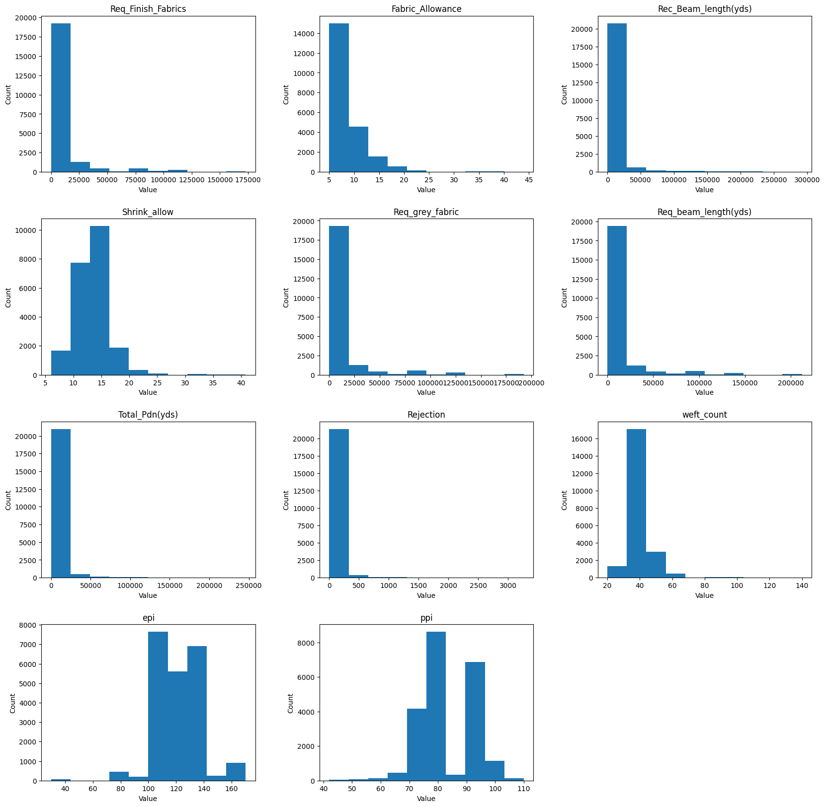
The next statement is again to visualize and it shows that in most columns there are outliers in the sequence that might skew the average of the values.

fig = plt.figure(figsize=[20, 20])
axes = dataset.hist(figsize=[20, 20], grid=False)
for ax in axes.flatten():
    ax.set_xlabel("Value")
    ax.set_ylabel("Count")
plt.show()

<Figure size 2000x2000 with 0 Axes>

#This finds the categorical data columns
for column in dataset.columns :
  if dataset[column].dtype == 'object':
    print(column)

Construction
Previous_pdn
warp_count

Find the trends and plot your data

To see how different values affect rejection

for column in dataset.columns :
  if dataset[column].dtype != 'object':
    dataset.plot(x='Rejection',y=column,kind='scatter')

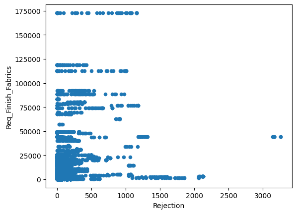
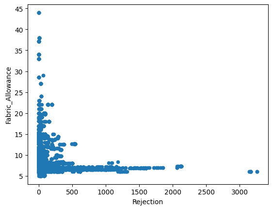
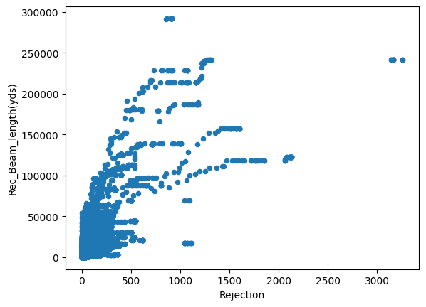
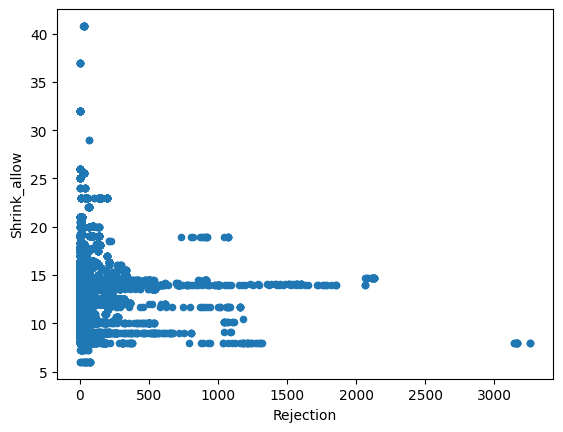
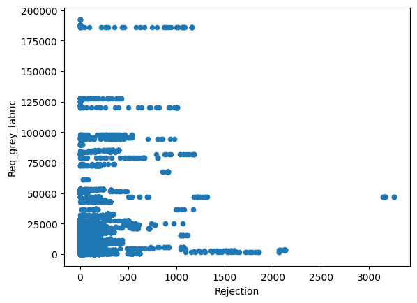
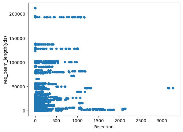
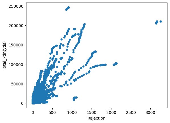
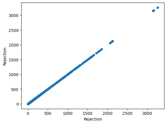
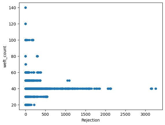
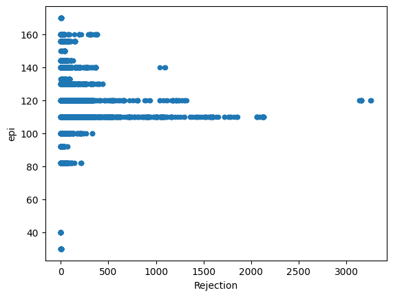
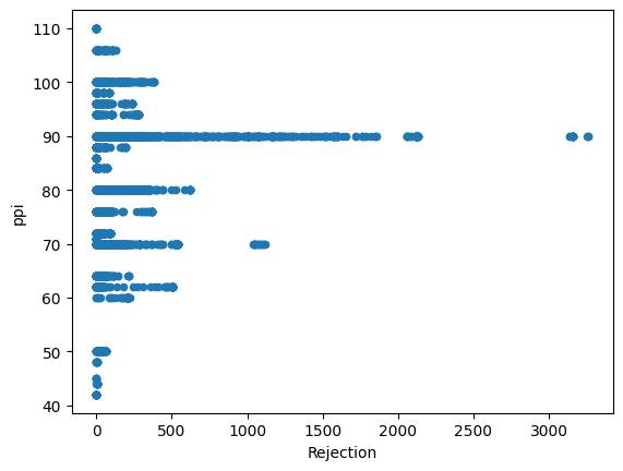
Just from visualizing the graph of data we can we can see rejection and Total_Pdn(yds) are directly proportional and so is the Rec_Beam_length(yds) and rejection,ie as Rec_Beam_length(yds)/Total_Pdn(yds) increases the rejection also increases.

#Step 2: Data Pre-processing Remove duplicate data

dataset.drop_duplicates(inplace=True)

dataset.shape

(10383, 14)

dataset.describe(include='O')

	Construction	Previous_pdn	warp_count
count	10383	10383	10383
unique	127	1	10
top	40x40/120x80	TOTAL	40
freq	1827	10383	7985

Dropping Extra Columns

Therefore the construction column was dropped as the categorical data was very unique and it would not help much in prediction of Rejection.

Previous_pdn has only one value which is was not going to help.

dataset.drop(["Construction","Previous_pdn"], axis = 1, inplace = True)

##Handling the warp count data

The column warp_count includes string data like ‘double_40’ which means that 2 threads of 40 count are weaved to make a single thread and that is weaved together to make the fabric.This is information can be useful to predict the rejection so instead of doubling 40 to replace all values with 80. We have introduced a new binary coloumn ‘is_double’ to keep track of using two threads while making the warp_count column numerical data.

dataset['thread_count'] = dataset['warp_count'].str.extract('(\d+)').astype(int)  # Extract numbers
dataset['is_double'] = dataset['warp_count'].str.contains('double').astype(int)  # Binary encoding
dataset.drop('warp_count', axis=1, inplace=True)
dataset

	Req_Finish_Fabrics	Fabric_Allowance	Rec_Beam_length(yds)	Shrink_allow	Req_grey_fabric	Req_beam_length(yds)	Total_Pdn(yds)	Rejection	weft_count	epi	ppi	thread_count	is_double
0	31300.0	6.0	38286.9360	12.5	33297.872340	34797.651103	27646.0	285	80.0	110	80	40	1
1	10450.0	7.0	13057.5840	14.5	11236.559140	12017.350432	11019.0	39	40.0	110	90	40	0
2	900.0	11.5	1902.8640	12.5	1016.949153	1062.753843	1528.0	0	40.0	110	80	40	0
3	8000.0	8.0	10093.9280	14.0	8695.652174	9245.815159	8944.0	58	40.0	130	80	40	0
4	3500.0	8.1	69146.1408	9.1	3808.487486	3831.158751	59367.0	1043	50.0	140	70	50	0
...	...	...	...	...	...	...	...	...	...	...	...	...	...
21970	1600.0	7.1	3597.9440	15.3	1722.282024	1859.355175	1388.0	16	40.0	120	80	40	0
21971	2400.0	8.4	3062.0800	14.5	2620.087336	2802.148531	249.0	12	40.0	130	80	40	0
21972	83449.0	7.0	20286.2800	10.2	89730.107527	91369.942153	5849.0	28	40.0	92	70	40	0
22003	83449.0	7.0	120.2960	10.2	89730.107527	91369.942153	85.0	0	40.0	110	90	40	0
22007	83449.0	7.0	131.2320	10.2	89730.107527	91369.942153	83.0	0	40.0	110	90	40	0

10383 rows × 13 columns

Heatmap to see correlation of data

fig, ax = plt.subplots(figsize=(12,9))
sns.heatmap(dataset.corr(method='pearson'),cmap="RdBu", annot=True,ax=ax,vmin=-1, vmax=1, center= 0);

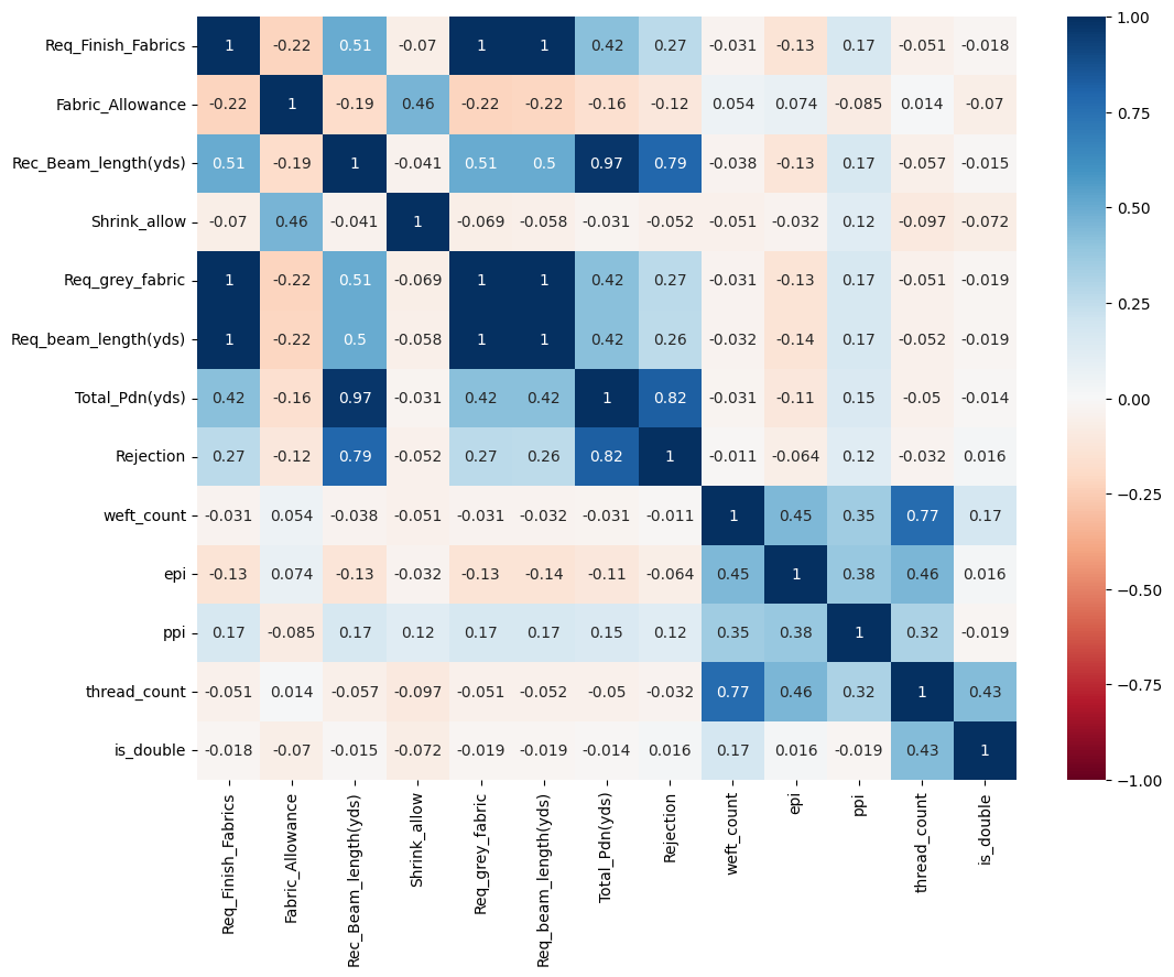
Req_grey_fabric and Req_beam_length(yds) have a perfectly positive correlation to Req_Finish_Fabrics hence I dropped it as in the heatmap the intersection values are 1.

dataset.drop(["Req_grey_fabric","Req_beam_length(yds)"], axis = 1, inplace = True)
dataset

#More information about this in conclusion
#dataset.drop(["Total_Pdn(yds)"])
#dataset.drop(["Rec_Beam_length(yds)"])

	Req_Finish_Fabrics	Fabric_Allowance	Rec_Beam_length(yds)	Shrink_allow	Total_Pdn(yds)	Rejection	weft_count	epi	ppi	thread_count	is_double
0	31300.0	6.0	38286.9360	12.5	27646.0	285	80.0	110	80	40	1
1	10450.0	7.0	13057.5840	14.5	11019.0	39	40.0	110	90	40	0
2	900.0	11.5	1902.8640	12.5	1528.0	0	40.0	110	80	40	0
3	8000.0	8.0	10093.9280	14.0	8944.0	58	40.0	130	80	40	0
4	3500.0	8.1	69146.1408	9.1	59367.0	1043	50.0	140	70	50	0
...	...	...	...	...	...	...	...	...	...	...	...
21970	1600.0	7.1	3597.9440	15.3	1388.0	16	40.0	120	80	40	0
21971	2400.0	8.4	3062.0800	14.5	249.0	12	40.0	130	80	40	0
21972	83449.0	7.0	20286.2800	10.2	5849.0	28	40.0	92	70	40	0
22003	83449.0	7.0	120.2960	10.2	85.0	0	40.0	110	90	40	0
22007	83449.0	7.0	131.2320	10.2	83.0	0	40.0	110	90	40	0

10383 rows × 11 columns

New heat map after dropping highly correlated coloumns

fig, ax = plt.subplots(figsize=(12,9))
sns.heatmap(dataset.corr(method='pearson'),cmap="RdBu", annot=True,ax=ax,vmin=-1, vmax=1, center= 0);

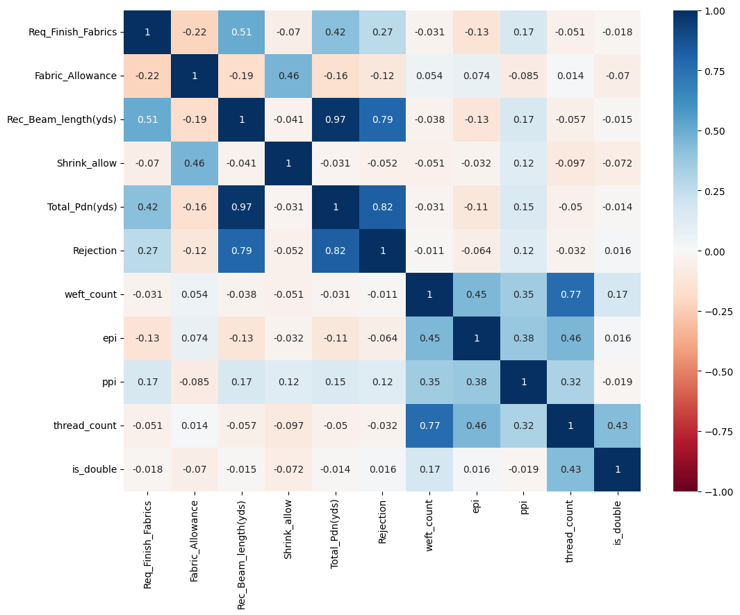
Checking the missing values

Finding no. of missing values

nandata=dataset.isnull().sum()
nandata

	0
Req_Finish_Fabrics	0
Fabric_Allowance	0
Rec_Beam_length(yds)	0
Shrink_allow	0
Total_Pdn(yds)	0
Rejection	0
weft_count	0
epi	0
ppi	0
thread_count	0
is_double	0

dtype: int64

There are no missing values in the data

##Splitting and Rearranging the dataset into the Training set and Test set

dataset.columns

Index(['Req_Finish_Fabrics', 'Fabric_Allowance', 'Rec_Beam_length(yds)',
       'Shrink_allow', 'Total_Pdn(yds)', 'Rejection', 'weft_count', 'epi',
       'ppi', 'thread_count', 'is_double'],
      dtype='object')

dataset=dataset[['Req_Finish_Fabrics', 'Fabric_Allowance', 'Rec_Beam_length(yds)','Shrink_allow',
                 'Total_Pdn(yds)','weft_count', 'epi','ppi', 'thread_count', 'is_double', 'Rejection']]

X = dataset.iloc[:, :-1]
y = dataset.iloc[:, -1]

X

	Req_Finish_Fabrics	Fabric_Allowance	Rec_Beam_length(yds)	Shrink_allow	Total_Pdn(yds)	weft_count	epi	ppi	thread_count	is_double
0	31300.0	6.0	38286.9360	12.5	27646.0	80.0	110	80	40	1
1	10450.0	7.0	13057.5840	14.5	11019.0	40.0	110	90	40	0
2	900.0	11.5	1902.8640	12.5	1528.0	40.0	110	80	40	0
3	8000.0	8.0	10093.9280	14.0	8944.0	40.0	130	80	40	0
4	3500.0	8.1	69146.1408	9.1	59367.0	50.0	140	70	50	0
...	...	...	...	...	...	...	...	...	...	...
21970	1600.0	7.1	3597.9440	15.3	1388.0	40.0	120	80	40	0
21971	2400.0	8.4	3062.0800	14.5	249.0	40.0	130	80	40	0
21972	83449.0	7.0	20286.2800	10.2	5849.0	40.0	92	70	40	0
22003	83449.0	7.0	120.2960	10.2	85.0	40.0	110	90	40	0
22007	83449.0	7.0	131.2320	10.2	83.0	40.0	110	90	40	0

10383 rows × 10 columns

y

	Rejection
0	285
1	39
2	0
3	58
4	1043
...	...
21970	16
21971	12
21972	28
22003	0
22007	0

10383 rows × 1 columns

dtype: int64

X_train, X_test, y_train, y_test = train_test_split(X, y, test_size = 0.2, random_state = 1)

This is a 80% training and 20% testing split

#Step 3: Training & Step 4: Evaluate

Linear Regression

regressor_mlr = LinearRegression()
regressor_mlr.fit(X_train, y_train)

LinearRegression()

In a Jupyter environment, please rerun this cell to show the HTML representation or trust the notebook.
On GitHub, the HTML representation is unable to render, please try loading this page with nbviewer.org.

y_pred = regressor_mlr.predict(X_test)
np.set_printoptions(precision=2)
print(np.concatenate(
    (y_pred.reshape(len(y_pred), 1), y_test.values.reshape(len(y_test), 1)), axis=1))

[[ 13.88   0.  ]
 [ 19.81 139.  ]
 [ 17.44  29.  ]
 ...
 [ 14.77   0.  ]
 [-89.88   0.  ]
 [133.31  54.  ]]

Combined the predicted values (y_pred) and actual values (y_test) side by side for comparison

plt.figure(figsize=(8, 6))
plt.scatter(y_test, y_pred, label='Actual vs. Predicted')
plt.plot([min(y_test), max(y_test)], [min(y_test), max(y_test)], linestyle='--', color='red', label='Perfect Prediction')  # Add a diagonal line for reference
plt.xlabel('Actual Rejection Rates')
plt.ylabel('Predicted Rejection Rates')
plt.title('Actual vs. Predicted Rejection Rates')
plt.legend()
plt.grid(True)
plt.show()

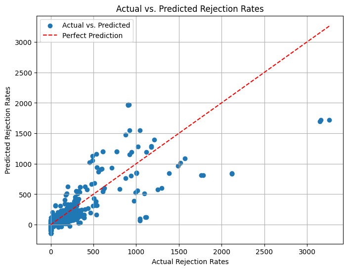
r2_score(y_test, y_pred)

0.6522871065814979

Accuracy:~65%

Polynomial Regression

poly_reg = PolynomialFeatures(degree = 3)
X_poly = poly_reg.fit_transform(X_train)
regressor_pr = LinearRegression()
regressor_pr.fit(X_poly, y_train)

LinearRegression()

In a Jupyter environment, please rerun this cell to show the HTML representation or trust the notebook.
On GitHub, the HTML representation is unable to render, please try loading this page with nbviewer.org.

y_pred = regressor_pr.predict(poly_reg.transform(X_test))
np.set_printoptions(precision=2)
print(np.concatenate((y_pred.reshape(len(y_pred), 1), y_test.values.reshape(len(y_test), 1)), axis=1))

[[ -8.66   0.  ]
 [ 70.94 139.  ]
 [  7.47  29.  ]
 ...
 [ 22.06   0.  ]
 [ 19.19   0.  ]
 [159.14  54.  ]]

plt.figure(figsize=(8, 6))
plt.scatter(y_test, y_pred, label='Actual vs. Predicted')
plt.plot([min(y_test), max(y_test)], [min(y_test), max(y_test)], linestyle='--', color='red', label='Perfect Prediction')  # Add a diagonal line for reference
plt.xlabel('Actual Rejection Rates')
plt.ylabel('Predicted Rejection Rates')
plt.title('Actual vs. Predicted Rejection Rates')
plt.legend()
plt.grid(True)
plt.show()

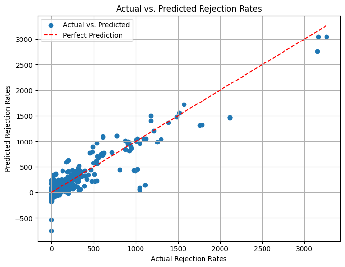
r2_score(y_test, y_pred)

0.8493012065564285

Improved accuracy:~85%

Support Vector Regression

Reference: https://www.coursera.org/specializations/machine-learning-introduction

regressor_svr = SVR(kernel = 'rbf') # Gaussian Radial basis function kernel
regressor_svr.fit(X_train, y_train)

SVR()

In a Jupyter environment, please rerun this cell to show the HTML representation or trust the notebook.
On GitHub, the HTML representation is unable to render, please try loading this page with nbviewer.org.

y_pred = regressor_svr.predict(X_test)
np.set_printoptions(precision=2)
print(np.concatenate((y_pred.reshape(len(y_pred), 1), y_test.values.reshape(len(y_test), 1)), axis=1))

[[  4.71   0.  ]
 [  8.58 139.  ]
 [  9.91  29.  ]
 ...
 [ -1.66   0.  ]
 [ 45.82   0.  ]
 [ 90.57  54.  ]]

Combined the predicted values (y_pred) and actual values (y_test) side by side for comparison

plt.figure(figsize=(8, 6))
plt.scatter(y_test, y_pred, label='Actual vs. Predicted')
plt.plot([min(y_test), max(y_test)], [min(y_test), max(y_test)], linestyle='--', color='red', label='Perfect Prediction')  # Add a diagonal line for reference
plt.xlabel('Actual Rejection Rates')
plt.ylabel('Predicted Rejection Rates')
plt.title('Actual vs. Predicted Rejection Rates')
plt.legend()
plt.grid(True)
plt.show()

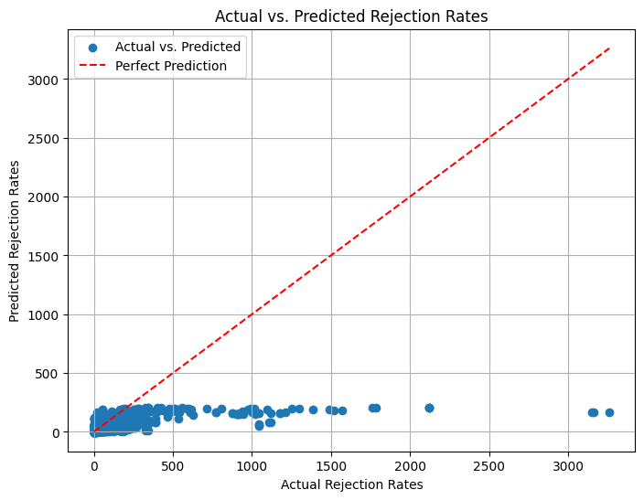
r2_score(y_test, y_pred)

0.18876622024345147

Very low accuracy:~19%

After Scaling

scaler = StandardScaler()
X_train_scaled = scaler.fit_transform(X_train)
X_test_scaled = scaler.transform(X_test)

regressor_svr = SVR(kernel = 'rbf')
regressor_svr.fit(X_train_scaled, y_train)

SVR()

In a Jupyter environment, please rerun this cell to show the HTML representation or trust the notebook.
On GitHub, the HTML representation is unable to render, please try loading this page with nbviewer.org.

y_pred = regressor_svr.predict(X_test_scaled)
np.set_printoptions(precision=2)
print(np.concatenate((y_pred.reshape(len(y_pred), 1), y_test.values.reshape(len(y_test), 1)), axis=1))

[[  3.54   0.  ]
 [ 30.33 139.  ]
 [  8.4   29.  ]
 ...
 [ 10.97   0.  ]
 [  7.01   0.  ]
 [ 55.65  54.  ]]

r2_score(y_test, y_pred)

0.09822515923462316

Lower accuracy:~10%

SVMs can struggle with complex relationships in data compared to polynomial regression, which explicitly models non-linear relationships. Our data has complex patterns,therefore SVM might underperform unless hyperparameters are finely tuned.

X_scaled = scaler.fit_transform(X)
svm_model = SVR(kernel='rbf', C=1, gamma=0.1)
scores = cross_val_score(svm_model, X_scaled, y, cv=5)
print(f"Mean CV Score: {scores.mean()}")

Mean CV Score: 0.18991249545238484

Accuracy:~19%

To confirm wheter the accuracy is low due to a certain train test split we try to get a more robust result using cross validation. However since the accuracy is still very low we can assume that the model is not a good fit for the data and is struggling with the complex relationships in the data.

Random Forest Regression

regressor_rfr = RandomForestRegressor(n_estimators = 2, random_state = 0, max_depth=5)
regressor_rfr.fit(X_train, y_train)

RandomForestRegressor(max_depth=5, n_estimators=2, random_state=0)

In a Jupyter environment, please rerun this cell to show the HTML representation or trust the notebook.
On GitHub, the HTML representation is unable to render, please try loading this page with nbviewer.org.

#y_pred = random_search.predict(X_test)
y_pred = regressor_rfr.predict(X_test)
np.set_printoptions(precision=2)
print(np.concatenate((y_pred.reshape(len(y_pred),1), y_test.values.reshape(len(y_test),1)),1))

[[  8.12   0.  ]
 [ 17.77 139.  ]
 [ 17.77  29.  ]
 ...
 [  1.39   0.  ]
 [ 13.06   0.  ]
 [117.97  54.  ]]

r2_score(y_test, y_pred)

0.9077670821517346

Non optimal Accuracy:~91%

The code for printing of the decision tree below has taken refrence from chat gpt

# Extract a single tree from the Random Forest
single_tree = regressor_rfr.estimators_[0]  # Pick the first tree

# Visualize using export_graphviz and graphviz
dot_data = export_graphviz(
    single_tree,
    out_file=None,  # Export directly as string
    feature_names=X_train.columns if hasattr(X_train, 'columns') else None,  # Use feature names if available
    filled=True,    # Color the nodes based on predictions
    rounded=True,   # Rounded corners for better readability
    special_characters=True
)

# Render the tree using graphviz
graph = graphviz.Source(dot_data)
graph.render("DecisionTree")  # Saves the visualization to a file called 'DecisionTree'
graph.view()                  # Open the file in your default viewer (or show inline in Jupyter)

# Inline visualization using plot_tree
plt.figure(figsize=(20, 10))  # Adjust size for readability
plot_tree(
    single_tree,
    feature_names=X_train.columns if hasattr(X_train, 'columns') else None,
    filled=True,
    rounded=True,
    fontsize=10
)
plt.show()

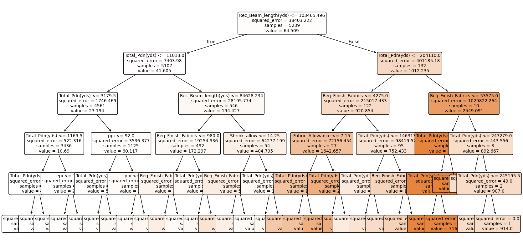
The above random forest model is only for easy visualisation purposes the actuaL OPTIMAL MODEL with greater accuracy is as below

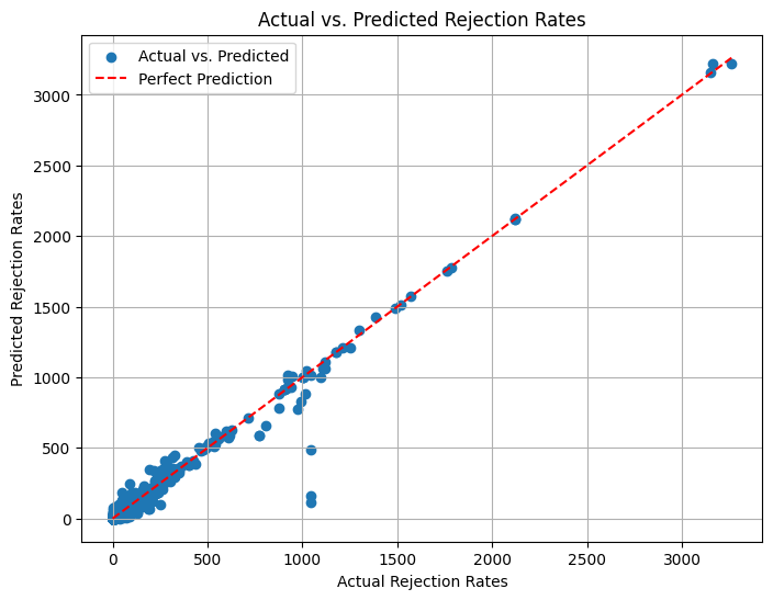
n_estimator chosen by trial and also keeping in mind not too overfit or increase complexity or time.Random_state is set to get consistent result

regressor_rfr = RandomForestRegressor(n_estimators = 200, random_state = 0)
regressor_rfr.fit(X_train, y_train)

####Method used for trial to find best n
# param_distributions = {
#     'n_estimators': [10, 50, 100, 200, 500],
#     'max_depth': [None, 10, 20],
# }

# random_search = RandomizedSearchCV(
#     estimator=RandomForestRegressor(random_state=0),
#     param_distributions=param_distributions,
#     scoring='neg_mean_squared_error',
#     n_iter=10,   # Number of parameter combinations to try
#     cv=3,        # Cross-validation folds
#     n_jobs=-1    # Use all available cores )

# print("Best Parameters:", random_search.best_params_)

RandomForestRegressor(n_estimators=200, random_state=0)

In a Jupyter environment, please rerun this cell to show the HTML representation or trust the notebook.
On GitHub, the HTML representation is unable to render, please try loading this page with nbviewer.org.

y_pred = regressor_rfr.predict(X_test)
np.set_printoptions(precision=2)
print(np.concatenate((y_pred.reshape(len(y_pred),1), y_test.values.reshape(len(y_test),1)),1))

[[  3.05   0.  ]
 [123.27 139.  ]
 [ 21.11  29.  ]
 ...
 [  0.14   0.  ]
 [  7.45   0.  ]
 [ 65.09  54.  ]]

plt.figure(figsize=(8, 6))
plt.scatter(y_test, y_pred, label='Actual vs. Predicted')
plt.plot([min(y_test), max(y_test)], [min(y_test), max(y_test)], linestyle='--', color='red', label='Perfect Prediction')  # Add a diagonal line for reference
plt.xlabel('Actual Rejection Rates')
plt.ylabel('Predicted Rejection Rates')
plt.title('Actual vs. Predicted Rejection Rates')
plt.legend()
plt.grid(True)
plt.show()

from sklearn.metrics import r2_score
r2_score(y_test, y_pred)

0.9718010479775304

Very good accuracy

Final Model with best accuracy without boosting

Accuracy:~ 97%

GradientBoostingRegressor Scikit

regressor_gbr = GradientBoostingRegressor(max_depth=5, n_estimators=500,learning_rate=0.05, random_state=42,criterion='friedman_mse')
regressor_gbr.fit(X_train, y_train)

GradientBoostingRegressor(learning_rate=0.05, max_depth=5, n_estimators=500,
                          random_state=42)

In a Jupyter environment, please rerun this cell to show the HTML representation or trust the notebook.
On GitHub, the HTML representation is unable to render, please try loading this page with nbviewer.org.

y_pred = regressor_gbr.predict(X_test)
np.set_printoptions(precision=2)
print(np.concatenate((y_pred.reshape(len(y_pred),1), y_test.values.reshape(len(y_test),1)),1))

[[  7.56   0.  ]
 [104.57 139.  ]
 [ 19.85  29.  ]
 ...
 [  2.18   0.  ]
 [  6.86   0.  ]
 [ 57.06  54.  ]]

plt.figure(figsize=(8, 6))
plt.scatter(y_test, y_pred, label='Actual vs. Predicted')
plt.plot([min(y_test), max(y_test)], [min(y_test), max(y_test)], linestyle='--', color='red', label='Perfect Prediction')  # Add a diagonal line for reference
plt.xlabel('Actual Rejection Rates')
plt.ylabel('Predicted Rejection Rates')
plt.title('Actual vs. Predicted Rejection Rates')
plt.legend()
plt.grid(True)
plt.show()

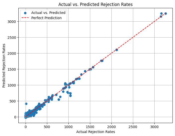
r2_score(y_test, y_pred)

0.9848724328476842

Improved accuracy:~98%

XGBRegressor

regressor_xg = XGBRegressor(max_depth=5,learning_rate=0.05,min_child_weight=2,n_estimators=500)
regressor_xg.fit(X_train, y_train)

XGBRegressor(base_score=None, booster=None, callbacks=None,
             colsample_bylevel=None, colsample_bynode=None,
             colsample_bytree=None, device=None, early_stopping_rounds=None,
             enable_categorical=False, eval_metric=None, feature_types=None,
             gamma=None, grow_policy=None, importance_type=None,
             interaction_constraints=None, learning_rate=0.05, max_bin=None,
             max_cat_threshold=None, max_cat_to_onehot=None,
             max_delta_step=None, max_depth=5, max_leaves=None,
             min_child_weight=2, missing=nan, monotone_constraints=None,
             multi_strategy=None, n_estimators=500, n_jobs=None,
             num_parallel_tree=None, random_state=None, ...)

In a Jupyter environment, please rerun this cell to show the HTML representation or trust the notebook.
On GitHub, the HTML representation is unable to render, please try loading this page with nbviewer.org.

parameters = {
    'n_estimators': [100, 200, 500],
    'max_depth':[2, 3, 5, 6],
    'learning_rate':[0.05,0.1,0.20],
    'min_child_weight':[1,2],
    'base_score':[0.25,0.5,0.75]
    }
random_cv = RandomizedSearchCV(estimator=regressor_xg,
            param_distributions=parameters,
            cv=5, n_iter=50,
            scoring = 'r2',n_jobs = -1,
            verbose = 0,
            return_train_score = True,
            random_state=0)
random_cv.fit(X_train,y_train)
random_cv.best_estimator_

XGBRegressor(base_score=0.5, booster=None, callbacks=None,
             colsample_bylevel=None, colsample_bynode=None,
             colsample_bytree=None, device=None, early_stopping_rounds=None,
             enable_categorical=False, eval_metric=None, feature_types=None,
             gamma=None, grow_policy=None, importance_type=None,
             interaction_constraints=None, learning_rate=0.2, max_bin=None,
             max_cat_threshold=None, max_cat_to_onehot=None,
             max_delta_step=None, max_depth=5, max_leaves=None,
             min_child_weight=2, missing=nan, monotone_constraints=None,
             multi_strategy=None, n_estimators=500, n_jobs=None,
             num_parallel_tree=None, random_state=None, ...)

In a Jupyter environment, please rerun this cell to show the HTML representation or trust the notebook.
On GitHub, the HTML representation is unable to render, please try loading this page with nbviewer.org.

y_pred = regressor_xg.predict(X_test)
np.set_printoptions(precision=2)
print(np.concatenate((y_pred.reshape(len(y_pred),1), y_test.values.reshape(len(y_test),1)),1))

[[  8.8    0.  ]
 [ 89.56 139.  ]
 [ 19.96  29.  ]
 ...
 [ -0.93   0.  ]
 [ 14.6    0.  ]
 [ 53.35  54.  ]]

plt.figure(figsize=(8, 6))
plt.scatter(y_test, y_pred, label='Actual vs. Predicted')
plt.plot([min(y_test), max(y_test)], [min(y_test), max(y_test)], linestyle='--', color='red', label='Perfect Prediction')  # Add a diagonal line for reference
plt.xlabel('Actual Rejection Rates')
plt.ylabel('Predicted Rejection Rates')
plt.title('Actual vs. Predicted Rejection Rates')
plt.legend()
plt.grid(True)
plt.show()

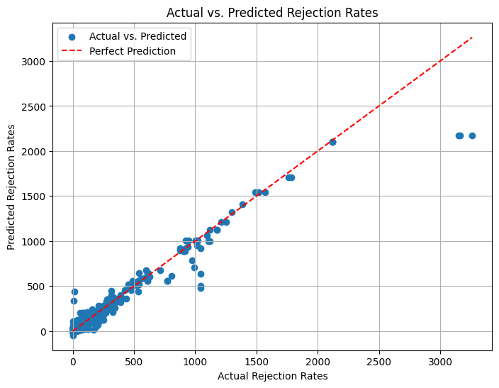
r2_score(y_test, y_pred)

0.9460485577583313

Decreased Accuracy:~ 95% maybe due to overfitting also we can see that we are getting negative values of y pred which do not really make sense

#Conclusion

The best accuracy was achived with the GradientBoostingRegressor Scikit. Best Accuracy:~98%

The findings very intresting which emphasize the importance of precise parameter control in minimizing rejections and improving production efficiency. Recommendations include optimizing recommended beam length and total production, which directly affect rejection rates. This analysis provides a robust framework for enhancing quality control and cost efficiency in textile manufacturing, serving as a foundation for data-driven process optimization.By testing dropping the recommended beam length column and total production, drastically decreased the accuracy which shows that they are key factors in predicting the weaving rejection.

#Reference links

https://www.geeksforgeeks.org/decision-tree-implementation-python/

https://stackoverflow.com/questions/72543209/how-to-use-a-gradientboostingregressor-in-scikit-learn-with-3-output-dimensions

https://machinelearningmastery.com/xgboost-for-regression/

baguirre2651/Citi-Bike-Demand-Prediction-Project-