Homework 5 (Due 11/1/2024 at 11:59pm)

Name:

ID:

Submission instruction:

• Download the file as .ipynb (see top right corner on the webpage).

• Write your name and ID in the field above.

• Answer the questions in the .ipynb file in either markdown or code cells.

• Before submission, make sure to rerun all cells by clicking Kernel -> Restart & Run All and check all the outputs.

• Upload the .ipynb file to Gradescope.

Q1 Linear regression on exponential growth

Suppose we want to measure the growth of a population of bacteria. We culture the bacteria in a test tube. We measure the volume of the cell culture at various times (hr) and obtain the following dataframe:

import pandas as pd
import seaborn as sns
import matplotlib.pyplot as plt

df_bac = pd.DataFrame({'time': [0, 1.5, 5, 9, 10], 'Volume':[0.37, 1.63, 2.4, 6.2, 10.66]})
print(df_bac)

   time  Volume
0   0.0    0.37
1   1.5    1.63
2   5.0    2.40
3   9.0    6.20
4  10.0   10.66

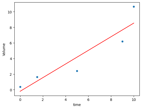
(1) Use linear regression to fit the data. Compute the \(R^2\). Plot the data and the fitted line on the same figure.

from sklearn.linear_model import LinearRegression
import numpy as np

sns.scatterplot(data=df_bac, x='time', y='Volume')

lm = LinearRegression()
lm.fit(df_bac[['time']], df_bac['Volume'])

sns.lineplot(x=df_bac['time'], y=lm.predict(df_bac[['time']]), color='red')

score = lm.score(df_bac[['time']], df_bac['Volume'])
print(f'R2' , score)

R2 0.8523390725174672

(2) We know that when nutrients are abundant, the bacteria grow exponentially. Therefore, a better model might be

\[ y = a e^{bx} \]

where \(y\) is the volume of the bacteria culture and \(x\) is the time.

Can we turn this into a linear regression problem?

Hint: Take the natural logarithm of both sides of the equation.

After taking the natural logarithm, we have

\[ \log y = \log a + bx \]

This is a linear regression problem.

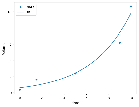
(3) After the transformation, find the optimal values of \(a\) and \(b\). Compute the \(R^2\). Plot the data and the fitted curve in the same figure. Is it better than the linear model?

# exponential growth
lm2 = LinearRegression()
lm2.fit(df_bac[['time']], np.log(df_bac['Volume']))
a = np.exp(lm2.intercept_)
b = lm2.coef_[0]

print(a, b)

# compute R2
y_pred = a * np.exp(b * df_bac['time'])
mse = np.mean((df_bac['Volume'] - y_pred) ** 2)
var = np.var(df_bac['Volume'])
r2 = 1 - mse / var
print('R2 = ', r2)
# the R2 is higher than the linear model


# plot the exponential fit
sns.scatterplot(data=df_bac, x='time', y='Volume')
xx = np.linspace(0, 10, 100)
yy = a * np.exp(b * xx)
sns.lineplot(x=xx, y=yy)
# add legend
_ = plt.legend(labels=["data","fit"])

0.5954551711492091 0.2805094137824158
R2 =  0.9605944747794366

Q2 Multiple linear regression

In this problem, we would like to predict the body_mass_g of a penguin based on the other features in the dataset.

# Do not modify this cell
df = sns.load_dataset("penguins")
df.dropna(inplace=True)

from sklearn.model_selection import train_test_split
# the stratify parameter makes sure that the train and test sets have the same proportion of species
df_train, df_test = train_test_split(df, test_size=0.5, random_state=0, stratify=df['species'])

In this exercise, Let’s consider what is the best subset of features to predict body_mass_g. This is called the best subset selection problem.

Since we have 3 features, we can fit 7 models, each with a different subset of features:

• Model 1: bill_length_mm

• Model 2: bill_depth_mm

• Model 3: flipper_length_mm

• Model 4: bill_length_mm, bill_depth_mm

• Model 5: bill_length_mm, flipper_length_mm

• Model 6: bill_depth_mm, flipper_length_mm

• Model 7: bill_length_mm, bill_depth_mm, flipper_length_mm

For each model, fit a linear regression model and compute the \(R^2\) on the training and testing data. Which model has the best \(R^2\) on the testing data? Is the best model the one with the most features?

# Feel free to use this variable. 
# all_subsets = [ ['bill_length_mm'], ['bill_depth_mm'], ['flipper_length_mm'], 
#                 ['bill_length_mm', 'bill_depth_mm'], ['bill_length_mm', 'flipper_length_mm'], ['bill_depth_mm', 'flipper_length_mm'], 
#                 ['bill_length_mm', 'bill_depth_mm', 'flipper_length_mm']]
# Alternatively, you can check out itertools.combinations (part of the Python standard library) to generate all combinations of a list

from itertools import combinations

features = ['bill_length_mm', 'bill_depth_mm',	'flipper_length_mm']

best_subset = []
best_score = 0

for L in range(1, len(features) + 1):
    for subset in combinations(features, L):
        lm = LinearRegression()
        lm.fit(df_train[list(subset)], df_train['body_mass_g'])
        test_score = lm.score(df_test[list(subset)], df_test['body_mass_g'])
        train_score = lm.score(df_train[list(subset)], df_train['body_mass_g'])

        print(f'{subset}: {train_score:.4f} {test_score:.4f}')

        if test_score > best_score:
            best_score = test_score
            best_subset = subset

print(f'best subset: {best_subset} {best_score:.4f}')

('bill_length_mm',): 0.3792 0.3101
('bill_depth_mm',): 0.2185 0.2134
('flipper_length_mm',): 0.7489 0.7731
('bill_length_mm', 'bill_depth_mm'): 0.4890 0.4385
('bill_length_mm', 'flipper_length_mm'): 0.7523 0.7689
('bill_depth_mm', 'flipper_length_mm'): 0.7508 0.7745
('bill_length_mm', 'bill_depth_mm', 'flipper_length_mm'): 0.7532 0.7705
best subset: ('bill_depth_mm', 'flipper_length_mm') 0.7745

Q3 Working with categorical variables

Let’s try to make use of the species feature in predicting the body_mass_g

# Do not modify this cell
df_penguins = sns.load_dataset("penguins")
df_penguins.dropna(inplace=True)

We can think of two different methods to encode the categorical feature:

1. Method 1: Using integer 1, 2, 3 …

2. Method 2: Using dummy variables such as is_category_A, where is_category_A is 1 if the category is A, 0 otherwise.

In this problem, we will compare the two methods.

For our dataset, the species are ['Adelie', 'Chinstrap', 'Gentoo'].

Let’s generate a few new features in df_penguins:

• code is 0 if the species is Adelie, 1 if the species is Chinstrap, 2 if the species is Gentoo

• is_Adelie is 1 if the species is Adelie, 0 otherwise

• is_Chinstrap is 1 if the species is Chinstrap, 0 otherwise

The is_Adelie and is_Chinstrap features are called dummy variables.

df_penguins['is_Adelie'] = df_penguins['species'] == 'Adelie'
df_penguins['is_Chinstrap'] = df_penguins['species'] == 'Chinstrap'

# encode species as 0 1 2
code = {'Adelie': 0, 'Chinstrap': 1, 'Gentoo': 2}
df_penguins['code'] = df_penguins['species'].map(code)

After generating these new features, split the new augmented dataframe into training and testing sets use the following command

# Do not modify this cell
df_penguins_train, df_penguins_test = train_test_split(df_penguins, test_size=0.5, random_state=0, stratify=df_penguins['species'])

(2) Compare the performance using different combinations of features. Compute the \(R^2\) on training and testing sets. Which one is the best?

• Baseline: ['bill_length_mm', 'bill_depth_mm', 'flipper_length_mm']

• Use code: ['bill_length_mm', 'bill_depth_mm', 'flipper_length_mm', 'code']

• Use dummy: ['bill_length_mm', 'bill_depth_mm', 'flipper_length_mm', 'is_Adelie', 'is_Chinstrap']

# we define a helper function for our workflow: take some features, fit a linear regression model, and return the R2 score
def get_score(df_train, df_test, features):
    lm = LinearRegression()
    lm.fit(df_train[features], df_train['body_mass_g'])
    train_score = lm.score(df_train[features], df_train['body_mass_g'])
    test_score = lm.score(df_test[features], df_test['body_mass_g'])
    return train_score, test_score

features = ['bill_length_mm', 'bill_depth_mm', 'flipper_length_mm']
train_score, test_score = get_score(df_penguins_train, df_penguins_test, features)
print(f'Baseline: Train score: {train_score:.3f}, Test score: {test_score:.3f}')


features = ['bill_length_mm', 'bill_depth_mm', 'flipper_length_mm', 'code']
train_score, test_score = get_score(df_penguins_train, df_penguins_test, features)
print(f'Use code: Train score: {train_score:.3f}, Test score: {test_score:.3f}')


features = ['bill_length_mm', 'bill_depth_mm', 'flipper_length_mm', 'is_Adelie', 'is_Chinstrap']
train_score, test_score = get_score(df_penguins_train, df_penguins_test, features)
print(f'Use dummy: Train score: {train_score:.3f}, Test score: {test_score:.3f}')

# the dummy variables are better than the code variable
# In general, encoding categorical variables as integers 1 2 3 is not a good idea, because it implies an order between the categories that does not exist.
# However, in some case, when the categories are age groups, it can make sense to encode them as 1 2 3, as there is an order between the categories.

Baseline: Train score: 0.753, Test score: 0.770
Use code: Train score: 0.763, Test score: 0.760
Use dummy: Train score: 0.851, Test score: 0.839