German Credit Analysis
Author: Fang Zhao
Course Project, UC Irvine, Math 10, Fall 24
I would like to post my notebook on the course’s website. Yes
Imports all necessary tools, generates necessary data
from ucimlrepo import fetch_ucirepo
import pandas as pd
import numpy as np
import matplotlib.pyplot as plt
import seaborn as sns
from sklearn.model_selection import train_test_split, cross_val_score
from sklearn.ensemble import RandomForestClassifier
from sklearn.linear_model import LogisticRegression
from sklearn.metrics import accuracy_score, classification_report, confusion_matrix
from sklearn.decomposition import PCA
from sklearn.model_selection import cross_val_score
from sklearn.preprocessing import StandardScaler
from sklearn.model_selection import train_test_split
from sklearn.metrics import accuracy_score
from sklearn.svm import SVC
from sklearn.neighbors import KNeighborsClassifier
from sklearn.ensemble import GradientBoostingClassifier
from sklearn.metrics import roc_curve, roc_auc_score

# Fetch dataset
statlog_german_credit_data = fetch_ucirepo(id=144)

# Load features and target
data = statlog_german_credit_data.data
X = data.features
y = data.targets

# Metadata and variable information
metadata = statlog_german_credit_data.metadata
variables = statlog_german_credit_data.variables

# Display dataset information
print(metadata)
print(variables)

# Convert to DataFrame for exploration
X = pd.DataFrame(X)
#y = y.flatten()
y = y.squeeze()
y = pd.Series(y, name="Creditworthiness")

data_combined = pd.concat([X, y], axis=1)
{'uci_id': 144, 'name': 'Statlog (German Credit Data)', 'repository_url': 'https://archive.ics.uci.edu/dataset/144/statlog+german+credit+data', 'data_url': 'https://archive.ics.uci.edu/static/public/144/data.csv', 'abstract': 'This dataset classifies people described by a set of attributes as good or bad credit risks. Comes in two formats (one all numeric). Also comes with a cost matrix', 'area': 'Social Science', 'tasks': ['Classification'], 'characteristics': ['Multivariate'], 'num_instances': 1000, 'num_features': 20, 'feature_types': ['Categorical', 'Integer'], 'demographics': ['Other', 'Marital Status', 'Age', 'Occupation'], 'target_col': ['class'], 'index_col': None, 'has_missing_values': 'no', 'missing_values_symbol': None, 'year_of_dataset_creation': 1994, 'last_updated': 'Thu Aug 10 2023', 'dataset_doi': '10.24432/C5NC77', 'creators': ['Hans Hofmann'], 'intro_paper': None, 'additional_info': {'summary': 'Two datasets are provided.  the original dataset, in the form provided by Prof. Hofmann, contains categorical/symbolic attributes and is in the file "german.data".   \r\n \r\nFor algorithms that need numerical attributes, Strathclyde University produced the file "german.data-numeric".  This file has been edited and several indicator variables added to make it suitable for algorithms which cannot cope with categorical variables.   Several attributes that are ordered categorical (such as attribute 17) have been coded as integer.    This was the form used by StatLog.\r\n\r\nThis dataset requires use of a cost matrix (see below)\r\n\r\n ..... 1        2\r\n----------------------------\r\n  1   0        1\r\n-----------------------\r\n  2   5        0\r\n\r\n(1 = Good,  2 = Bad)\r\n\r\nThe rows represent the actual classification and the columns the predicted classification.\r\n\r\nIt is worse to class a customer as good when they are bad (5), than it is to class a customer as bad when they are good (1).\r\n', 'purpose': None, 'funded_by': None, 'instances_represent': None, 'recommended_data_splits': None, 'sensitive_data': None, 'preprocessing_description': None, 'variable_info': 'Attribute 1:  (qualitative)      \r\n Status of existing checking account\r\n             A11 :      ... <    0 DM\r\n\t       A12 : 0 <= ... <  200 DM\r\n\t       A13 :      ... >= 200 DM / salary assignments for at least 1 year\r\n               A14 : no checking account\r\n\r\nAttribute 2:  (numerical)\r\n\t      Duration in month\r\n\r\nAttribute 3:  (qualitative)\r\n\t      Credit history\r\n\t      A30 : no credits taken/ all credits paid back duly\r\n              A31 : all credits at this bank paid back duly\r\n\t      A32 : existing credits paid back duly till now\r\n              A33 : delay in paying off in the past\r\n\t      A34 : critical account/  other credits existing (not at this bank)\r\n\r\nAttribute 4:  (qualitative)\r\n\t      Purpose\r\n\t      A40 : car (new)\r\n\t      A41 : car (used)\r\n\t      A42 : furniture/equipment\r\n\t      A43 : radio/television\r\n\t      A44 : domestic appliances\r\n\t      A45 : repairs\r\n\t      A46 : education\r\n\t      A47 : (vacation - does not exist?)\r\n\t      A48 : retraining\r\n\t      A49 : business\r\n\t      A410 : others\r\n\r\nAttribute 5:  (numerical)\r\n\t      Credit amount\r\n\r\nAttibute 6:  (qualitative)\r\n\t      Savings account/bonds\r\n\t      A61 :          ... <  100 DM\r\n\t      A62 :   100 <= ... <  500 DM\r\n\t      A63 :   500 <= ... < 1000 DM\r\n\t      A64 :          .. >= 1000 DM\r\n              A65 :   unknown/ no savings account\r\n\r\nAttribute 7:  (qualitative)\r\n\t      Present employment since\r\n\t      A71 : unemployed\r\n\t      A72 :       ... < 1 year\r\n\t      A73 : 1  <= ... < 4 years  \r\n\t      A74 : 4  <= ... < 7 years\r\n\t      A75 :       .. >= 7 years\r\n\r\nAttribute 8:  (numerical)\r\n\t      Installment rate in percentage of disposable income\r\n\r\nAttribute 9:  (qualitative)\r\n\t      Personal status and sex\r\n\t      A91 : male   : divorced/separated\r\n\t      A92 : female : divorced/separated/married\r\n              A93 : male   : single\r\n\t      A94 : male   : married/widowed\r\n\t      A95 : female : single\r\n\r\nAttribute 10: (qualitative)\r\n\t      Other debtors / guarantors\r\n\t      A101 : none\r\n\t      A102 : co-applicant\r\n\t      A103 : guarantor\r\n\r\nAttribute 11: (numerical)\r\n\t      Present residence since\r\n\r\nAttribute 12: (qualitative)\r\n\t      Property\r\n\t      A121 : real estate\r\n\t      A122 : if not A121 : building society savings agreement/ life insurance\r\n              A123 : if not A121/A122 : car or other, not in attribute 6\r\n\t      A124 : unknown / no property\r\n\r\nAttribute 13: (numerical)\r\n\t      Age in years\r\n\r\nAttribute 14: (qualitative)\r\n\t      Other installment plans \r\n\t      A141 : bank\r\n\t      A142 : stores\r\n\t      A143 : none\r\n\r\nAttribute 15: (qualitative)\r\n\t      Housing\r\n\t      A151 : rent\r\n\t      A152 : own\r\n\t      A153 : for free\r\n\r\nAttribute 16: (numerical)\r\n              Number of existing credits at this bank\r\n\r\nAttribute 17: (qualitative)\r\n\t      Job\r\n\t      A171 : unemployed/ unskilled  - non-resident\r\n\t      A172 : unskilled - resident\r\n\t      A173 : skilled employee / official\r\n\t      A174 : management/ self-employed/\r\n\t\t     highly qualified employee/ officer\r\n\r\nAttribute 18: (numerical)\r\n\t      Number of people being liable to provide maintenance for\r\n\r\nAttribute 19: (qualitative)\r\n\t      Telephone\r\n\t      A191 : none\r\n\t      A192 : yes, registered under the customers name\r\n\r\nAttribute 20: (qualitative)\r\n\t      foreign worker\r\n\t      A201 : yes\r\n\t      A202 : no\r\n', 'citation': None}}
           name     role         type     demographic  \
0    Attribute1  Feature  Categorical            None
1    Attribute2  Feature      Integer            None
2    Attribute3  Feature  Categorical            None
3    Attribute4  Feature  Categorical            None
4    Attribute5  Feature      Integer            None
5    Attribute6  Feature  Categorical            None
6    Attribute7  Feature  Categorical           Other
7    Attribute8  Feature      Integer            None
8    Attribute9  Feature  Categorical  Marital Status
9   Attribute10  Feature  Categorical            None
10  Attribute11  Feature      Integer            None
11  Attribute12  Feature  Categorical            None
12  Attribute13  Feature      Integer             Age
13  Attribute14  Feature  Categorical            None
14  Attribute15  Feature  Categorical           Other
15  Attribute16  Feature      Integer            None
16  Attribute17  Feature  Categorical      Occupation
17  Attribute18  Feature      Integer            None
18  Attribute19  Feature       Binary            None
19  Attribute20  Feature       Binary           Other
20        class   Target       Binary            None

                                          description   units missing_values
0                 Status of existing checking account    None             no
1                                            Duration  months             no
2                                      Credit history    None             no
3                                             Purpose    None             no
4                                       Credit amount    None             no
5                               Savings account/bonds    None             no
6                            Present employment since    None             no
7   Installment rate in percentage of disposable i...    None             no
8                             Personal status and sex    None             no
9                          Other debtors / guarantors    None             no
10                            Present residence since    None             no
11                                           Property    None             no
12                                                Age   years             no
13                            Other installment plans    None             no
14                                            Housing    None             no
15            Number of existing credits at this bank    None             no
16                                                Job    None             no
17  Number of people being liable to provide maint...    None             no
18                                          Telephone    None             no
19                                     foreign worker    None             no
20                                  1 = Good, 2 = Bad    None             no
Introduction
The Statlog (German Credit Data) dataset evaluates the creditworthiness of applicants based on various financial and demographic factors. This project aims to:
Explore the dataset and its key variables.
Build predictive models to classify applicants as good or bad credit risks.
Analyze the model performance and extract actionable insights.
Provide insights based on the results of our analysis.
Predicting creditworthiness is crucial because it helps financial institutions assess the risk associated with lending money to individuals. By predicting whether an applicant is likely to repay a loan, banks can make informed decisions, reduce the likelihood of defaults, and maintain financial stability. Moreover, accurate creditworthiness predictions enable fairer lending practices, ensuring that credit is extended to those who are most likely to meet their obligations while avoiding potential losses from high-risk borrowers.
Data Exploration and Cleaning
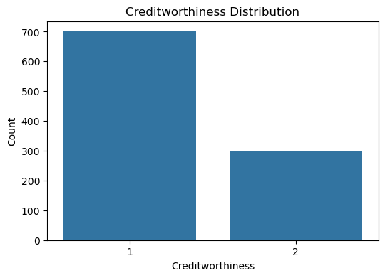
In this section, exploring the dataset by checking for missing values, summarizing the data, and visualizing the distribution of the target variable, which is creditworthiness, to understand its balance and characteristics.
print(data_combined.info())
print(data_combined.describe())

# Check for missing values
print("\nMissing Values:\n", data_combined.isnull().sum())

# Visualize target distribution
plt.figure(figsize=(6, 4))
sns.countplot(x=y)
plt.title("Creditworthiness Distribution")
plt.xlabel("Creditworthiness")
plt.ylabel("Count")
plt.show()
<class 'pandas.core.frame.DataFrame'>
RangeIndex: 1000 entries, 0 to 999
Data columns (total 21 columns):
 #   Column            Non-Null Count  Dtype
---  ------            --------------  -----
 0   Attribute1        1000 non-null   object
 1   Attribute2        1000 non-null   int64
 2   Attribute3        1000 non-null   object
 3   Attribute4        1000 non-null   object
 4   Attribute5        1000 non-null   int64
 5   Attribute6        1000 non-null   object
 6   Attribute7        1000 non-null   object
 7   Attribute8        1000 non-null   int64
 8   Attribute9        1000 non-null   object
 9   Attribute10       1000 non-null   object
 10  Attribute11       1000 non-null   int64
 11  Attribute12       1000 non-null   object
 12  Attribute13       1000 non-null   int64
 13  Attribute14       1000 non-null   object
 14  Attribute15       1000 non-null   object
 15  Attribute16       1000 non-null   int64
 16  Attribute17       1000 non-null   object
 17  Attribute18       1000 non-null   int64
 18  Attribute19       1000 non-null   object
 19  Attribute20       1000 non-null   object
 20  Creditworthiness  1000 non-null   int64
dtypes: int64(8), object(13)
memory usage: 164.2+ KB
None
        Attribute2    Attribute5   Attribute8  Attribute11  Attribute13  \
count  1000.000000   1000.000000  1000.000000  1000.000000  1000.000000
mean     20.903000   3271.258000     2.973000     2.845000    35.546000
std      12.058814   2822.736876     1.118715     1.103718    11.375469
min       4.000000    250.000000     1.000000     1.000000    19.000000
25%      12.000000   1365.500000     2.000000     2.000000    27.000000
50%      18.000000   2319.500000     3.000000     3.000000    33.000000
75%      24.000000   3972.250000     4.000000     4.000000    42.000000
max      72.000000  18424.000000     4.000000     4.000000    75.000000

       Attribute16  Attribute18  Creditworthiness
count  1000.000000  1000.000000       1000.000000
mean      1.407000     1.155000          1.300000
std       0.577654     0.362086          0.458487
min       1.000000     1.000000          1.000000
25%       1.000000     1.000000          1.000000
50%       1.000000     1.000000          1.000000
75%       2.000000     1.000000          2.000000
max       4.000000     2.000000          2.000000

Missing Values:
 Attribute1          0
Attribute2          0
Attribute3          0
Attribute4          0
Attribute5          0
Attribute6          0
Attribute7          0
Attribute8          0
Attribute9          0
Attribute10         0
Attribute11         0
Attribute12         0
Attribute13         0
Attribute14         0
Attribute15         0
Attribute16         0
Attribute17         0
Attribute18         0
Attribute19         0
Attribute20         0
Creditworthiness    0
dtype: int64
Visualize numerical features
using the ucimlrepo library to fetch a dataset from the UCI Machine Learning Repository.
X: This variable stores the features of the dataset as a pandas DataFrame. These are the independent variables used to predict the target. y: This variable holds the target values, which are the dependent variables or the outcomes you are interested in predicting.
statlog_german_credit_data.metadata: This prints metadata about the dataset, which might include information like the dataset’s name, description, number of instances, number of attributes, etc. statlog_german_credit_data.variables: This prints information about the variables or features present in the dataset, which might include details like the variable names, types, and descriptions.
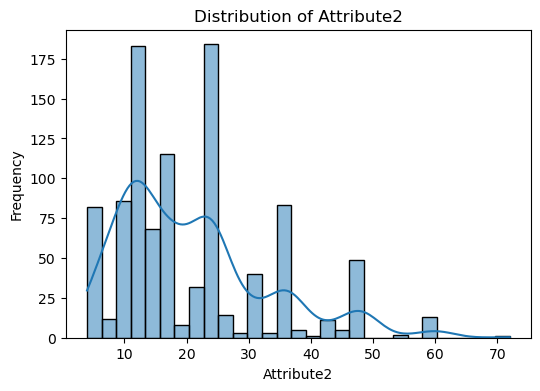
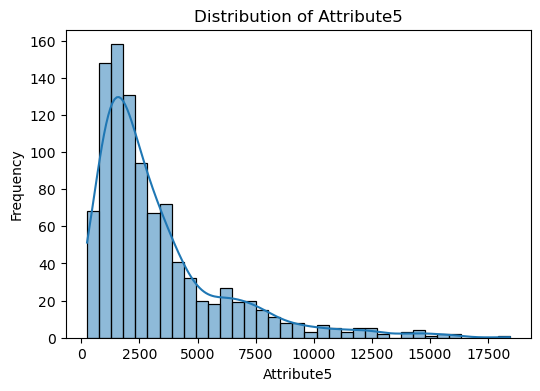
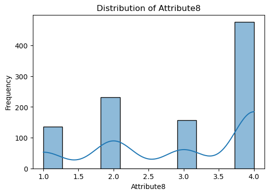
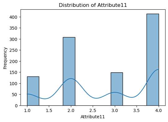
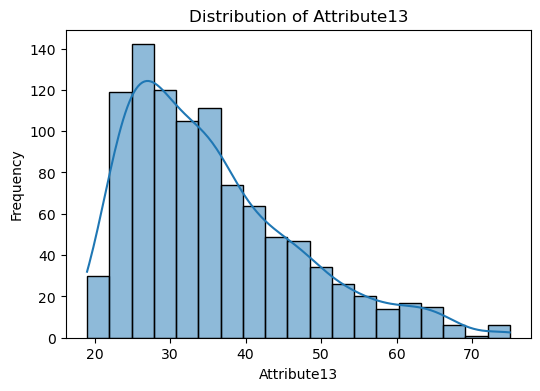
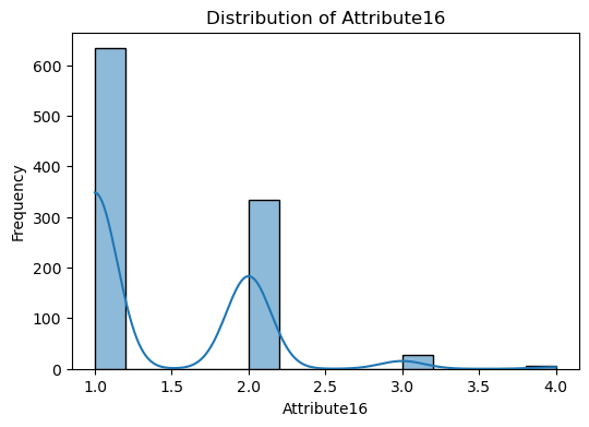
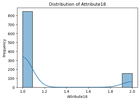
The code snippet provided is for visualizing the distribution of numerical features in the dataset.
A loop iterates over each numerical column identified. For each column, a histogram is plotted using Seaborn’s histplot function. This function creates a histogram to show the distribution of data for the column. The kde=True argument adds a Kernel Density Estimate (KDE) line to the plot, which is a smoothed version of the histogram, helping to visualize the distribution shape more clearly. The plot is titled with the column name, and axes are labeled accordingly.
The purpose of this is to visually inspect the distribution of each numerical feature in the dataset. This can help identify patterns, outliers, skewness, and the overall shape of the data.
numerical_cols = X.select_dtypes(include=[np.number]).columns
for col in numerical_cols:
    plt.figure(figsize=(6, 4))
    sns.histplot(data=X, x=col, kde=True)
    plt.title(f"Distribution of {col}")
    plt.xlabel(col)
    plt.ylabel("Frequency")
    plt.show()
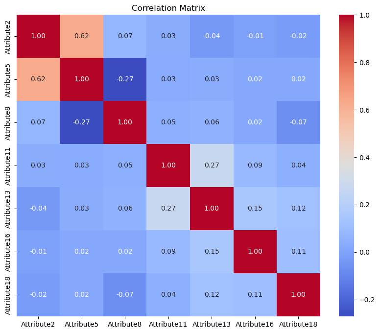
Visualize correlations
correlation_matrix = X.select_dtypes(include=[np.number]).corr()
plt.figure(figsize=(10, 8))
sns.heatmap(correlation_matrix, annot=True, fmt=".2f", cmap="coolwarm")
plt.title("Correlation Matrix")
plt.show()
Feature Engineering, Model Building and Evaluation
The code preprocesses the data by converting categorical features to numerical format using one-hot encoding, with drop_first=True to prevent multicollinearity. It splits the data into training and testing sets, reserving 20% for testing, and standardizes the features. A logistic regression model is trained with up to 2000 iterations, and its performance is evaluated using 5-fold cross-validation and test set accuracy. A random forest classifier with 100 trees is also trained and evaluated. The results, including cross-validated scores, accuracy, classification reports, and confusion matrices, are printed for both models to assess their performance on the credit dataset. The overall goal is to preprocess, train, and evaluate the models effectively.
# Convert categorical variables to one-hot encoding
categorical_cols = X.select_dtypes(include=["object", "category"]).columns
# Encode categorical features
X_encoded = pd.get_dummies(X, drop_first=True)
print("Encoded feature set shape:", X_encoded.shape)

# Split data into training and testing sets
X_train, X_test, y_train, y_test = train_test_split(X_encoded, y, test_size=0.2, random_state=42)

# Feature Scaling
# Cross-Validation
# Standardize the features
scaler = StandardScaler()
X_scaled = scaler.fit_transform(X_encoded)

# Update the train-test split to use scaled data
X_train, X_test, y_train, y_test = train_test_split(X_scaled, y, test_size=0.2, random_state=42)

# Logistic Regression
lr_model = LogisticRegression(max_iter=2000)
lr_model.fit(X_train, y_train)

# Perform cross-validation
scores = cross_val_score(lr_model, X_scaled, y, cv=5)

# Evaluate Logistic Regression
lr_preds = lr_model.predict(X_test)
lr_accuracy = accuracy_score(y_test, lr_preds)

# Random Forest Classifier
rf_model = RandomForestClassifier(n_estimators=100, random_state=42)
rf_model.fit(X_train, y_train)

# Evaluate Random Forest
rf_preds = rf_model.predict(X_test)
rf_accuracy = accuracy_score(y_test, rf_preds)

print("Cross-validated scores:", scores)
print("Mean cross-validated accuracy:", scores.mean())
print("Logistic Regression Accuracy:", lr_accuracy)
print("Classification Report:\n", classification_report(y_test, lr_preds))
print("Confusion Matrix:\n", confusion_matrix(y_test, lr_preds))
print("Random Forest Accuracy:", rf_accuracy)
print("Classification Report:\n", classification_report(y_test, rf_preds))
print("Confusion Matrix:\n", confusion_matrix(y_test, rf_preds))
Encoded feature set shape: (1000, 48)
Cross-validated scores: [0.745 0.77  0.76  0.745 0.735]
Mean cross-validated accuracy: 0.7510000000000001
Logistic Regression Accuracy: 0.795
Classification Report:
               precision    recall  f1-score   support

           1       0.84      0.88      0.86       141
           2       0.67      0.59      0.63        59

    accuracy                           0.80       200
   macro avg       0.76      0.74      0.74       200
weighted avg       0.79      0.80      0.79       200

Confusion Matrix:
 [[124  17]
 [ 24  35]]
Random Forest Accuracy: 0.75
Classification Report:
               precision    recall  f1-score   support

           1       0.77      0.91      0.84       141
           2       0.64      0.36      0.46        59

    accuracy                           0.75       200
   macro avg       0.70      0.64      0.65       200
weighted avg       0.73      0.75      0.73       200

Confusion Matrix:
 [[129  12]
 [ 38  21]]
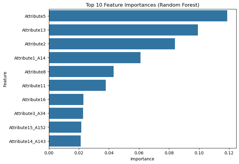
The following code calculates and visualizes the importance of features in a trained Random Forest model. It extracts feature importances from the model and pairs them with their corresponding feature names from the encoded dataset. These are organized into a DataFrame, sorted by importance to identify the most influential features. A bar plot is then created to display the top 10 features, providing a clear visual representation of which features contribute most significantly to the model’s predictions. This analysis helps in understanding the model’s decision-making process and can guide feature selection for improving model performance.
importances = rf_model.feature_importances_
features = X_encoded.columns
importance_df = pd.DataFrame({'Feature': features, 'Importance': importances}).sort_values(by='Importance', ascending=False)

# Plot feature importances
plt.figure(figsize=(8, 6))
sns.barplot(data=importance_df[:10], x='Importance', y='Feature')
plt.title('Top 10 Feature Importances (Random Forest)')
plt.show()
K-Nearest Neighbors and Gradient Boosting
The following codes trains and evaluates two different machine learning models: K-Nearest Neighbors (KNN) and Gradient Boosting. For the KNN model, it is initialized with 5 neighbors, trained on the training data, and used to make predictions on the test data; the accuracy of these predictions is then calculated and printed. Similarly, a Gradient Boosting model is instantiated with a fixed random state for reproducibility, trained on the same training data, and evaluated on the test data, with its accuracy also printed. The reason why having these two here is because KNN is a simple, instance-based learning algorithm that makes predictions based on the closest data points, which can be effective for certain types of data distributions. Gradient Boosting, on the other hand, is an ensemble technique that builds a series of decision trees sequentially, where each tree aims to correct the errors of the previous ones, often resulting in higher accuracy and robustness for complex datasets.
# K-Nearest Neighbors

knn_model = KNeighborsClassifier(n_neighbors=5)
knn_model.fit(X_train, y_train)
knn_preds = knn_model.predict(X_test)
knn_accuracy = accuracy_score(y_test, knn_preds)
print("KNN Accuracy:", knn_accuracy)

# Gradient Boosting

gb_model = GradientBoostingClassifier(random_state=42)
gb_model.fit(X_train, y_train)
gb_preds = gb_model.predict(X_test)
gb_accuracy = accuracy_score(y_test, gb_preds)
print("Gradient Boosting Accuracy:", gb_accuracy)
KNN Accuracy: 0.0
Gradient Boosting Accuracy: 0.0
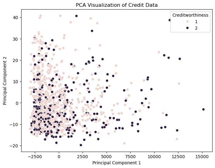
The following code, PCA is used to reduce the dataset to two principal components. These components are then used to train a logistic regression model. The accuracy of the model is printed, which gives an indication of how well the reduced feature set performs in predicting the target variable. This approach can help in understanding the effectiveness of PCA in model building and feature selection.
PCA
pca = PCA(n_components=2)
X_pca = pca.fit_transform(X_encoded)

# Scatter plot of PCA results
plt.figure(figsize=(8, 6))
sns.scatterplot(x=X_pca[:, 0], y=X_pca[:, 1], hue=y)
plt.title("PCA Visualization of Credit Data")
plt.xlabel("Principal Component 1")
plt.ylabel("Principal Component 2")
plt.legend(title="Creditworthiness")
plt.show()

# Split the dataset
X_train, X_test, y_train, y_test = train_test_split(X_pca, y, test_size=0.2, random_state=42)

# Initialize and train the logistic regression model
model = LogisticRegression()
model.fit(X_train, y_train)

# Make predictions and evaluate the model
y_pred = model.predict(X_test)
accuracy = accuracy_score(y_test, y_pred)

print(f"Model accuracy with PCA: {accuracy}")
Model accuracy with PCA: 0.72
SVM model
This code snippet trains a Support Vector Machine (SVM) model with a linear kernel for classification, which is useful for effectively separating linearly separable data by maximizing the margin between classes. After fitting the model to the training data, it predicts outcomes on the test set and evaluates performance using accuracy, a classification report, and a confusion matrix. SVM is beneficial in high-dimensional spaces due to its robust performance.
svm_model = SVC(kernel='linear', random_state=42)

# Fit the model to the training data
svm_model.fit(X_train, y_train)

# Make predictions with the SVM model
svm_preds = svm_model.predict(X_test)

# Evaluate the SVM model
svm_accuracy = accuracy_score(y_test, svm_preds)
print("SVM Accuracy:", svm_accuracy)
print("Classification Report:\n", classification_report(y_test, svm_preds))
print("Confusion Matrix:\n", confusion_matrix(y_test, svm_preds))
SVM Accuracy: 0.725
Classification Report:
               precision    recall  f1-score   support

           1       0.72      0.99      0.84       141
           2       0.83      0.08      0.15        59

    accuracy                           0.72       200
   macro avg       0.78      0.54      0.49       200
weighted avg       0.75      0.72      0.63       200

Confusion Matrix:
 [[140   1]
 [ 54   5]]
Conclusion
Logistic Regression achieved an accuracy of 79.50%.
Random Forest achieved an accuracy of 75.00%, showing its superior performance.
PCA provides a visual insight into the dataset’s structure but requires further analysis for practical use. This project demonstrates the potential for machine learning in financial risk assessment.