Linear Regression#
Problem#
Given the training dataset \(x_i\in\mathbb{R}\), \(y_i\in\mathbb{R}\), \(i= 1,2,..., N\), we want to find the linear function
that fits the relations between \(x_i\) and \(y_i\). So that given any \(x\), we can make the prediction
Loss Function and Optimization#
With the training dataset, define the loss function \(L(w,b)\) of parameter \(w\) and \(b\), which is also called mean squared error (MSE)
where \(\hat{y}^{(i)}\) denotes the predicted value of y at \(x_i\), i.e. \(\hat{y}^{(i)} = wx_i+b\).
Our goal is to find the optimal \(w\) and \(b\) that minimize the loss function \(L(w,b)\), i.e.
This is a function of \(w\) and \(b\), and we can analytically solve \(\partial_{w}L = \partial_{b}L =0\), and yields
where \(\bar{X}\) and \(\bar{Y}\) are the mean of \(x\) and of \(y\), and \(\text{Cov}(X,Y)\) denotes the estimated covariance (or called sample covariance) between \(X\) and \(Y\), \(\text{Var}(Y)\) denotes the sample variance of \(Y\).
Evaluating the Model#
Mean Squared Error (MSE): Smaller MSE indicates better performance. However, MSE depends on the units of measurement—for example, changing units from meters to millimeters multiplies the MSE by a factor of \(1000^2\).
Coefficient of Determination \( R^{2} \):
\[ R^{2} = 1 - \frac{\sum_{i=1}^{N}(y_i-\hat{y}_i)^{2}}{\sum_{i=1}^{N}(y_i-\bar{y})^{2}} = 1 - \frac{\text{MSE}}{\text{Var}(Y)} \]A higher \( R^{2} \) (closer to 1) indicates better performance. Unlike MSE, \( R^{2} \) is dimensionless and independent of the units.
\( R^{2} \) measures the proportion of variance in the data explained by the model. If the model perfectly fits the data (MSE=0), then \( R^{2}=1 \). Conversely, using a constant model (predicting the mean), MSE equals the variance of \( y \), and \( R^{2}=0 \).
import numpy as np
import matplotlib.pyplot as plt

class myLinearRegression:
    '''
    The single-variable linear regression estimator.
    This serves as an example of the regression models from sklearn, with methods fit, predict, and score.
    '''
    def __init__(self):
        '''
        '''
        self.w = None
        self.b = None

    def fit(self, x, y):
        # covariance matrix,
        # bias = True makes the factor 1/N, otherwise 1/(N-1)
        # but it doesn't matter here, since the factor will be cancelled out in the calculation of w

        cov_mat = np.cov(x, y, bias=True)
        # cov_mat[0, 1] is the covariance of x and y, and cov_mat[0, 0] is the variance of x

        self.w = cov_mat[0, 1] / cov_mat[0, 0]
        self.b = np.mean(y) - self.w * np.mean(x)

        # :.3f means 3 decimal places
        print(f'w = {self.w:.3f}, b = {self.b:.3f}')

    def predict(self, x):
        '''
        Predict the output values for the input value x, based on trained parameters

        '''
        ypred = self.w * x + self.b
        return ypred

    def score(self, x, y):
        '''
        Calculate the R^2 score of the model
        '''
        mse =  np.mean((y - self.predict(x))**2)
        var = np.mean((y - np.mean(y))**2)
        Rsquare = 1 - mse / var
        return Rsquare
We can also use LinearRegression from sklearn.linear_model to fit the linear model.
# Use the following command to install scikit-learn
# %conda install scikit-learn
# or
# %pip install scikit-learn
# Generate synthetic data
np.random.seed(0) # for reproducibility
a = 0
b = 2
N = 200 # number of samples
sigma = 1 # noise level
x = np.random.uniform(a,b,(N,1))
y = 2 * x + 1 + np.random.normal(0, sigma, (N, 1))
y_gt = 2 * x + 1
# Fit the model
lm = LinearRegression()
lm.fit(x, y)
score = lm.score(x, y)
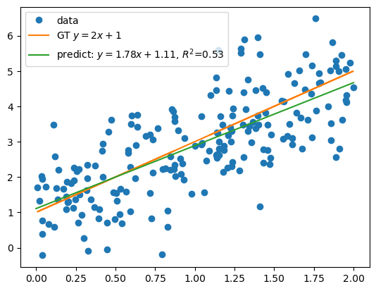
# plot data
plt.plot(x, y, 'o', label='data')
# plot ground truth
plt.plot(x, y_gt, label=f'GT $y=2x+1$')
# plot the linear regression model
xs = np.linspace(a, b, 100).reshape(-1, 1)
plt.plot(xs, lm.predict(xs), label=f'predict: $y={lm.coef_.item():.2f}x+{lm.intercept_.item():.2f}$, $R^2$={score:.2f}')
plt.legend()
score = 0.528
from sklearn.linear_model import LinearRegression

reg = LinearRegression()

# x need to be n-sample by p features
reg.fit(x.reshape(-1, 1), y)
print(f'w = {reg.coef_.item():.3f}, b = {reg.intercept_.item():.3f}')

score = reg.score(x.reshape(-1, 1), y)
print(f'score = {score:.3f}')
w = 1.781, b = 1.107
score = 0.528
What is the effect of centering the data?#
When \(X\) is centered, the slope \(w\) remains the same, but the intercept \(b\) changes.
The intercept now means the predicted Y when X is at the mean.
x_center = x - np.mean(x)

reg.fit(x_center.reshape(-1, 1), y)
print(f'w = {reg.coef_.item():.3f}, b = {reg.intercept_.item():.3f}')
score = reg.score(x_center.reshape(-1, 1), y)
print(f'score = {score:.3f}')
w = 1.781, b = 2.889
score = 0.528
What is the effect of scaling the data?#
When \(cX\) is used, the optimal slope is now \(w/c\), and the intercept does not change
scale_factor = 10
x_scale = x * scale_factor
reg.fit(x_scale.reshape(-1, 1), y)
print(f'w = {reg.coef_.item():.3f}, b = {reg.intercept_.item():.3f}')
score = reg.score(x_scale.reshape(-1, 1), y)
print(f'score = {score:.3f}')
w = 0.178, b = 1.107
score = 0.528
For linear regression, centering and scaling the data does not affect the performance of the model.
For some other models, centering and scaling can be essential
What is the best constant model?#
What is the best constant \(b\) that minimizes the loss function \(L(b)\)?
To solve \(\partial_{b}L = 0\),
where \(\bar{y}\) is the mean of \(y\).
Thus, the best constant model is
Appendix#
Detailed Derivation of the Optimal Parameters (Not exam material).
The loss function for simple linear regression is given by:
To find the optimal ( w ), we set the partial derivative of ( L ) with respect to ( w ) to zero:
Differentiate with respect to ( w ):
Rearrange this equation to get:
Derivative with respect to \(b\):
This simplifies to:
Or, equivalently:
Substitute \(b\) back into the equation (*), we get:
Expanding this:
Rearranging terms
Now, solving for \(w\):
Recall that \(Cov(X,Y) = E[XY]-E[X]E[Y]\), and \(Var(X) = E[X^2] - E[X]^2\). Divide both the numerator and the denominator by \(N\). We can rewrite the above equation in terms of covariance and variance: $\(w = \frac{Cov(X,Y)}{Var(X)}\)$
This is the final expression for \(w^*\) in simple linear regression, representing the slope of the best-fit line.