Week 4, Wed, 4/23

import numpy as np
import pandas as pd

# A synthetic dataset

N = 100
X = np.random.rand(N,2)
# y = 1 + 2 x_1 + 3 x_2
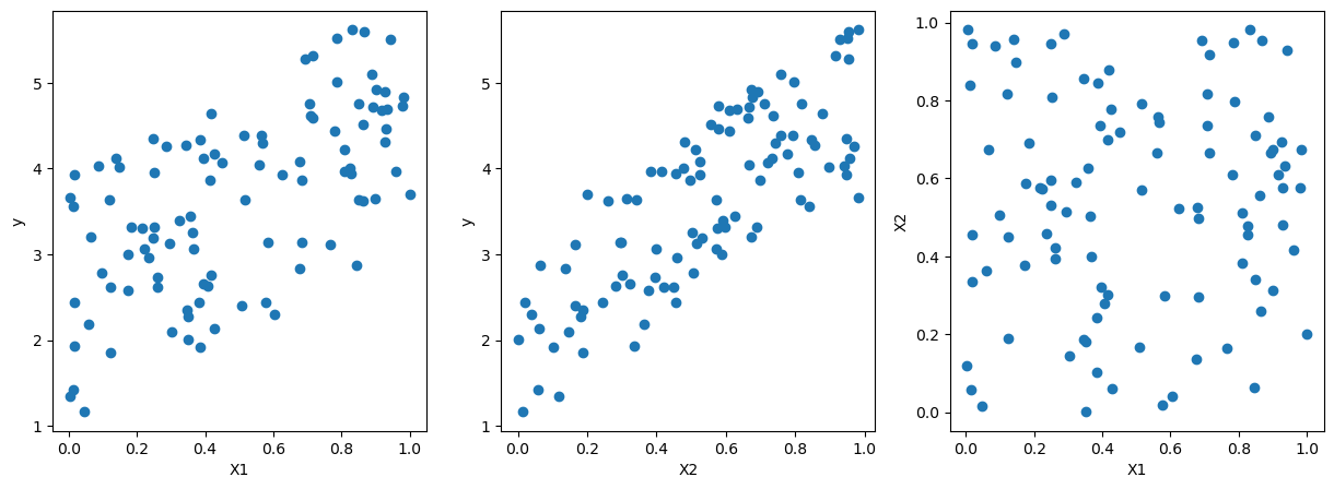
y = 1 + 2*X[:,0] + 3*X[:,1] + np.random.normal(0,0.1,N)

df = pd.DataFrame({'X1':X[:,0],'X2':X[:,1],'y':y})

df

	X1	X2	y
0	0.863820	0.260710	3.629063
1	0.826831	0.454714	3.948601
2	0.123193	0.188948	1.850269
3	0.780613	0.610546	4.444845
4	0.012375	0.840044	3.566947
...	...	...	...
95	0.999957	0.201042	3.696460
96	0.322909	0.589567	3.389103
97	0.624948	0.523743	3.934405
98	0.350681	0.180042	2.280561
99	0.849586	0.709870	4.762332

100 rows × 3 columns

import plotly.graph_objs as go
import plotly.express as px

# Create 3D scatter plot
fig = px.scatter_3d(df, x='X1', y='X2', z='y')

# Show interactive plot
fig.show()

import matplotlib.pyplot as plt

# pairwise scatter plot of X1, X2, y
fig, ax = plt.subplots(1,3,figsize=(15,5))
ax[0].scatter(X[:,0],y)
ax[0].set_xlabel('X1')
ax[0].set_ylabel('y')

ax[1].scatter(X[:,1],y)
ax[1].set_xlabel('X2')
ax[1].set_ylabel('y')

ax[2].scatter(X[:,0],X[:,1])
ax[2].set_xlabel('X1')
ax[2].set_ylabel('X2')

Text(0, 0.5, 'X2')

from sklearn import linear_model

lreg_sklearn = linear_model.LinearRegression()

lreg_sklearn.fit(X,y) 

LinearRegression()

In a Jupyter environment, please rerun this cell to show the HTML representation or trust the notebook.
On GitHub, the HTML representation is unable to render, please try loading this page with nbviewer.org.

print(lreg_sklearn.intercept_, lreg_sklearn.coef_)

1.0535067030741847 [1.99274839 2.92111383]

# Assuming coefficients and intercept from the sklearn linear regression model
coefficients = lreg_sklearn.coef_
intercept = lreg_sklearn.intercept_

# Create meshgrid for the regression plane
xx, yy = np.meshgrid(np.linspace(0, 1, 10), np.linspace(0, 1, 10))
zz = coefficients[0] * xx + coefficients[1] * yy + intercept

# Create the scatter plot for the data points
scatter = go.Scatter3d(
    x=X[:, 0],
    y=X[:, 1],
    z=y,
    mode='markers',
    marker=dict(size=5, color='blue'),
    name='Data Points'
)

# Create the surface plot for the regression plane
surface = go.Surface(
    x=xx,
    y=yy,
    z=zz,
    colorscale='reds',
    opacity=0.5,
    name='Regression Plane'
)

# Create the layout
layout = go.Layout(
    title='3D Plot of Data Points and Regression Plane',
    scene=dict(
        xaxis_title='X_1',
        yaxis_title='X_2',
        zaxis_title='Y'
    )
)

# Combine the scatter and surface plots
fig = go.Figure(data=[scatter, surface], layout=layout)

# Show the plot
fig.show()

import seaborn as sns

df = sns.load_dataset('penguins')
df.dropna(inplace=True)
df

	species	island	bill_length_mm	bill_depth_mm	flipper_length_mm	body_mass_g	sex
0	Adelie	Torgersen	39.1	18.7	181.0	3750.0	Male
1	Adelie	Torgersen	39.5	17.4	186.0	3800.0	Female
2	Adelie	Torgersen	40.3	18.0	195.0	3250.0	Female
4	Adelie	Torgersen	36.7	19.3	193.0	3450.0	Female
5	Adelie	Torgersen	39.3	20.6	190.0	3650.0	Male
...	...	...	...	...	...	...	...
338	Gentoo	Biscoe	47.2	13.7	214.0	4925.0	Female
340	Gentoo	Biscoe	46.8	14.3	215.0	4850.0	Female
341	Gentoo	Biscoe	50.4	15.7	222.0	5750.0	Male
342	Gentoo	Biscoe	45.2	14.8	212.0	5200.0	Female
343	Gentoo	Biscoe	49.9	16.1	213.0	5400.0	Male

333 rows × 7 columns

X = df[['bill_length_mm',	'bill_depth_mm',	'flipper_length_mm']]
X

	bill_length_mm	bill_depth_mm	flipper_length_mm
0	39.1	18.7	181.0
1	39.5	17.4	186.0
2	40.3	18.0	195.0
4	36.7	19.3	193.0
5	39.3	20.6	190.0
...	...	...	...
338	47.2	13.7	214.0
340	46.8	14.3	215.0
341	50.4	15.7	222.0
342	45.2	14.8	212.0
343	49.9	16.1	213.0

333 rows × 3 columns

y =  df['body_mass_g']

y

0      3750.0
1      3800.0
2      3250.0
4      3450.0
5      3650.0
        ...  
338    4925.0
340    4850.0
341    5750.0
342    5200.0
343    5400.0
Name: body_mass_g, Length: 333, dtype: float64

lreg_sklearn = linear_model.LinearRegression()

lreg_sklearn.fit(X,y)

LinearRegression()

In a Jupyter environment, please rerun this cell to show the HTML representation or trust the notebook.
On GitHub, the HTML representation is unable to render, please try loading this page with nbviewer.org.

lreg_sklearn.score(X,y)

0.7639366781169294

Colinearity

If two variables are highly correlated, intuitively, we can say that they are measuring the same thing. In the context of linear regression, this is called multicollinearity.

Suppose \(Y = aX_1\) and \(X_2 = bX_1\), then we can write \(Y = \beta_1 X_1 + \beta_2 X_2\) for any \(\beta_1\) and \(\beta_2\) such that \(\beta_1 + b \beta_2 = a\).

We can see that the coefficients are not unique.

This cause a few problems:

1. Interpretation: it’s difficult to interpret the coefficients. Originally, we would say that a one unit increase in \(X_1\) would lead to a \(\beta_1\) increase in \(Y\). But now, we can’t say that, because we can’t change \(X_1\) without changing \(X_2\).

2. Large Variance of the parameter: Since there could be infinite solutions, there is no guarantee which one the solver will find. Therefore small changes in the data could lead to large changes in the coefficients.

3. Numerical Stability: Sometimes the solver can’t find the solution.

However, this does not affect the prediction: even though the coefficients are not unique, the prediction will be the same.

import numpy as np
from sklearn.linear_model import LinearRegression


X = np.random.uniform(0,1,(100,1))
X = np.column_stack((X, X[:,0]*2))
y = X[:,0] + np.random.randn(X.shape[0]) * 0.1

# regression with X0 and X1
lreg_sklearn = LinearRegression()
lreg_sklearn.fit(X,y)
score = lreg_sklearn.score(X,y)
print(f'coefs using X0 and X1: {lreg_sklearn.coef_}, intercept: {lreg_sklearn.intercept_}, score: {score}')


# regression with X0
lreg_sklearn.fit(X[:,0:1],y)
score = lreg_sklearn.score(X[:,0:1],y)
print(f'coefs using X0: {lreg_sklearn.coef_}, intercept: {lreg_sklearn.intercept_}, score: {score}')

coefs using X0 and X1: [0.19438571 0.38877142], intercept: 0.013947482462746907, score: 0.879023539153949
coefs using X0: [0.97192856], intercept: 0.013947482462746963, score: 0.879023539153949