Week 3, Fri, 4/18

import seaborn as sns
import numpy as np
df = sns.load_dataset("penguins")

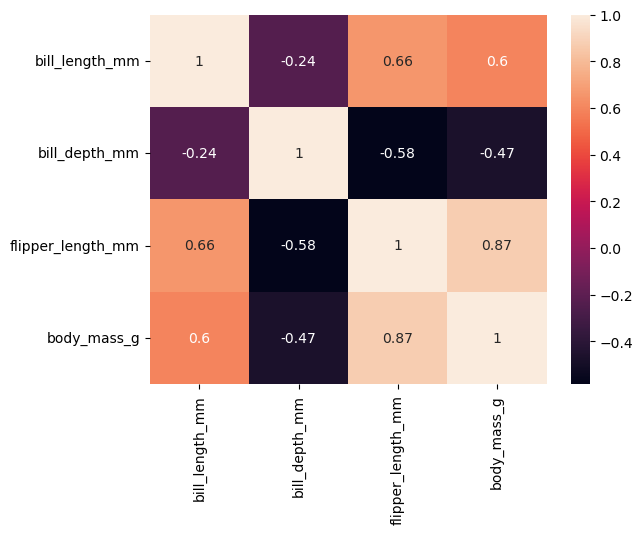
corr = df[["bill_length_mm", "bill_depth_mm", "flipper_length_mm", "body_mass_g"]].corr()
corr

	bill_length_mm	bill_depth_mm	flipper_length_mm	body_mass_g
bill_length_mm	1.000000	-0.235053	0.656181	0.595110
bill_depth_mm	-0.235053	1.000000	-0.583851	-0.471916
flipper_length_mm	0.656181	-0.583851	1.000000	0.871202
body_mass_g	0.595110	-0.471916	0.871202	1.000000

sns.heatmap(corr, annot=True)

<Axes: >

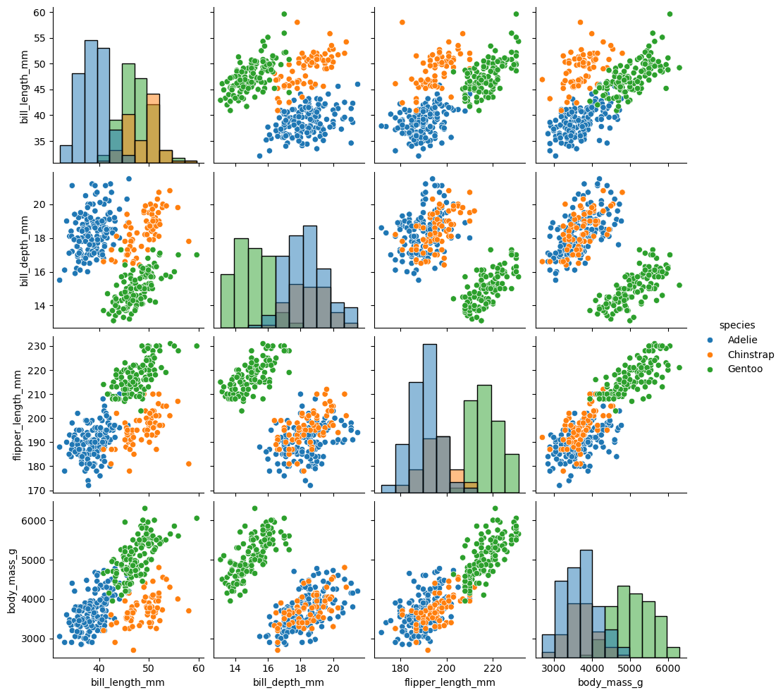
sns.pairplot(df, diag_kind="hist", hue = 'species')

<seaborn.axisgrid.PairGrid at 0x177f2e0c0>

Problem

Given the training dataset \(x_i\in\mathbb{R}\), \(y_i\in\mathbb{R}\), \(i= 1,2,..., N\), we want to find the linear function

\[ y\approx f(x) = wx + b \]

that fits the relations between \(x_i\) and \(y_i\). So that given any \(x\), we can make the prediction

\[ \hat{y} = f(x) = w x+b \]

Loss Function and Optimization

With the training dataset, define the loss function \(L(w,b)\) of parameter \(w\) and \(b\), which is also called mean squared error (MSE)

\[L(w,b)=\frac{1}{N}\sum_{i=1}^N\big(\hat{y}^{(i)}-y_i\big)^2=\frac{1}{N}\sum_{i=1}^N\big((wx_i+b)-y_i\big)^2,\]

where \(\hat{y}^{(i)}\) denotes the predicted value of y at \(x_i\), i.e. \(\hat{y}^{(i)} = wx_i+b\).

Our goal is to find the optimal \(w\) and \(b\) that minimize the loss function \(L(w,b)\), i.e.

\[\min_{w,b} L(w,b)\]

This is a function of \(w\) and \(b\), and we can analytically solve \(\partial_{w}L = \partial_{b}L =0\), and yields

\[w^* = \frac{\sum_{i=1}^{N} (x_i - \bar{X})(y_i - \bar{Y})}{\sum_{i=1}^{N} (x_i - \bar{X})^2} = \frac{\text{Cov}(X,Y)}{\text{Var}(X)}\]

\[b^* = \bar{Y} - w^*\bar{X}\]

where \(\bar{X}\) and \(\bar{Y}\) are the mean of \(x\) and of \(y\), and \(\text{Cov}(X,Y)\) denotes the estimated covariance (or called sample covariance) between \(X\) and \(Y\), \(\text{Var}(Y)\) denotes the sample variance of \(Y\).

# poll: What is the optimal slope and intercept for the data?
import numpy as np
x = np.array([0,1,2,3])
y = np.array([0,2,0,6])
cov_mat = np.cov(x,y)

cov_mat = np.cov(x,y,bias=False)
print(cov_mat)

[[1.66666667 2.66666667]
 [2.66666667 8.        ]]

cov_mat = np.cov(x,y,bias=True)
print(cov_mat)

[[1.25 2.  ]
 [2.   6.  ]]

w = cov_mat[0,1]/cov_mat[0,0]
w

1.6

b = np.mean(y) - w * np.mean(x)
b

-0.40000000000000036

Evaluating the Model

• Mean Squared Error (MSE): Smaller MSE indicates better performance. However, MSE depends on the units of measurement—for example, changing units from meters to millimeters multiplies the MSE by a factor of \(1000^2\).

• Coefficient of Determination \( R^{2} \): $\( R^{2} = 1 - \frac{\sum_{i=1}^{N}(y_i-\hat{y}_i)^{2}}{\sum_{i=1}^{N}(y_i-\bar{y})^{2}} = 1 - \frac{\text{MSE}}{\text{Var}(Y)} \)$

  A higher \( R^{2} \) (closer to 1) indicates better performance. Unlike MSE, \( R^{2} \) is dimensionless and independent of the units.

  \( R^{2} \) measures the proportion of variance in the data explained by the model. If the model perfectly fits the data (MSE=0), then \( R^{2}=1 \). Conversely, using a constant model (predicting the mean), MSE equals the variance of \( y \), and \( R^{2}=0 \).

import numpy as np
import matplotlib.pyplot as plt

class myLinearRegression:
    '''
    The single-variable linear regression estimator.
    This serves as an example of the regression models from sklearn, with methods fit, predict, and score.
    '''
    def __init__(self):
        '''
        '''
        self.w = None
        self.b = None
    
    def fit(self, x, y):
        # covariance matrix, 
        # bias = True makes the factor 1/N, otherwise 1/(N-1)
        # but it doesn't matter here, since the factor will be cancelled out in the calculation of w
        
        cov_mat = np.cov(x, y, bias=True)
        # cov_mat[0, 1] is the covariance of x and y, and cov_mat[0, 0] is the variance of x

        self.w = cov_mat[0, 1] / cov_mat[0, 0]
        self.b = np.mean(y) - self.w * np.mean(x)

        # :.3f means 3 decimal places
        print(f'w = {self.w:.3f}, b = {self.b:.3f}')

    def predict(self, x):
        '''
        Predict the output values for the input value x, based on trained parameters

        '''
        ypred = self.w * x + self.b
        return ypred

    def score(self, x, y):
        '''
        Calculate the R^2 score of the model
        '''
        mse =  np.mean((y - self.predict(x))**2)
        var = np.mean((y - np.mean(y))**2)
        Rsquare = 1 - mse / var
        return Rsquare