Week 2, Wed, 4/9

import numpy as np
import matplotlib.pyplot as plt
import seaborn as sns

n = 1000000
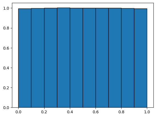
x = np.random.uniform(0, 1, n)
plt.hist(x, bins=10, edgecolor='black', density=True)

(array([0.99501098, 0.99885098, 1.00212099, 1.00326099, 1.00070099,
        1.00075099, 1.00176099, 1.00128099, 0.99957098, 0.99670098]),
 array([3.20964129e-07, 1.00000222e-01, 2.00000124e-01, 3.00000025e-01,
        3.99999927e-01, 4.99999828e-01, 5.99999730e-01, 6.99999631e-01,
        7.99999533e-01, 8.99999434e-01, 9.99999336e-01]),
 <BarContainer object of 10 artists>)

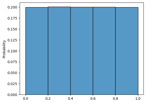
sns.histplot(x, bins=5, edgecolor='black', stat='probability')

<Axes: ylabel='Probability'>

import numpy as np
import matplotlib.pyplot as plt
import seaborn as sns

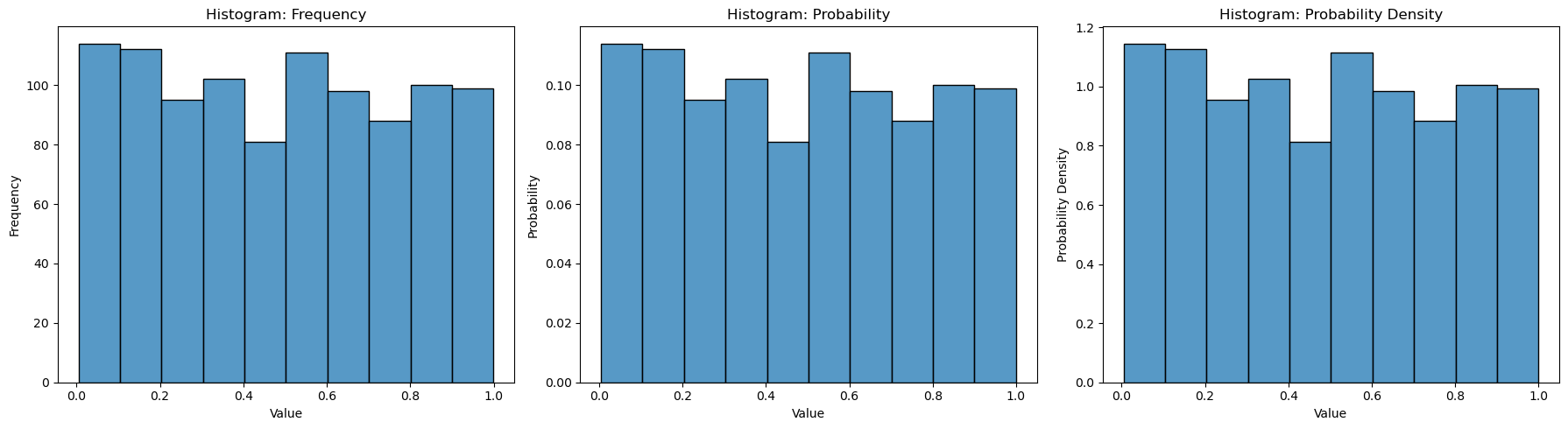
# Generate data from a uniform distribution
np.random.seed(42)
N = 1000
data = np.random.uniform(0, 1, N)
nbins = 10

# Create a 1x3 figure to show different types of histograms
fig, axs = plt.subplots(1, 3, figsize=(18, 5))

# Plot histogram showing frequency
# axs[0].hist(data, bins=20, edgecolor='black')
sns.histplot(data, bins=nbins, edgecolor='black', ax=axs[0])
axs[0].set_title('Histogram: Frequency')
axs[0].set_xlabel('Value')
axs[0].set_ylabel('Frequency')

# show probability
#  bar heights sum to 1
sns.histplot(data, bins=nbins, edgecolor='black', stat='probability', ax=axs[1])
axs[1].set_title('Histogram: Probability')
axs[1].set_xlabel('Value')
axs[1].set_ylabel('Probability')

# Plot histogram showing probability density
#  area under the histogram sums to 1
sns.histplot(data, bins=nbins, edgecolor='black', stat='density', ax=axs[2])
axs[2].set_title('Histogram: Probability Density')
axs[2].set_xlabel('Value')
axs[2].set_ylabel('Probability Density')



# Adjust layout and display the plot
plt.tight_layout()
plt.show()

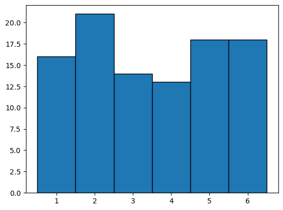
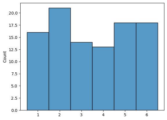
n = 100
x = np.random.randint(1, 7, n)
x

array([4, 6, 3, 5, 1, 5, 6, 6, 1, 2, 1, 4, 3, 2, 1, 5, 2, 2, 1, 2, 5, 6,
       2, 6, 5, 1, 3, 2, 3, 5, 2, 6, 4, 3, 2, 3, 2, 1, 6, 3, 4, 4, 5, 2,
       3, 5, 3, 2, 4, 1, 4, 5, 6, 1, 5, 2, 1, 5, 2, 4, 6, 2, 3, 2, 2, 6,
       3, 5, 5, 2, 3, 3, 6, 4, 5, 6, 1, 5, 6, 5, 4, 1, 4, 1, 2, 6, 1, 4,
       5, 1, 6, 1, 3, 5, 6, 6, 2, 4, 2, 6])

plt.hist(x, bins=6, range=(0.5, 6.5),edgecolor='black')

(array([16., 21., 14., 13., 18., 18.]),
 array([0.5, 1.5, 2.5, 3.5, 4.5, 5.5, 6.5]),
 <BarContainer object of 6 artists>)

sns.histplot(x,discrete=True)

<Axes: ylabel='Count'>

N = 10000
x = np.random.randint(1,7, (N,3))

max_each_round = x.max(axis=1)

max_each_round>4

array([ True, False, False, ...,  True,  True, False])

np.sum(max_each_round>4)/N

0.7074

(x.max(axis=1)>4).sum()/N

0.7074

N = 1000
x = np.random.uniform(0,1,size=(N,1))
y = np.random.uniform(0,1,size=(N,1))

r = np.sqrt(x**2+y**2)

(r<1).sum()/N

0.763

inside = r <= 1
plt.scatter(x[inside], y[inside], color='blue', alpha=0.5)
plt.scatter(x[~inside], y[~inside], color='red', alpha=0.5)
plt.axis('equal')

(-0.04960800372068671,
 1.048686021119046,
 -0.04554278212617771,
 1.0453759840903212)

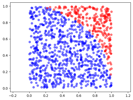
np.pi/4

0.7853981633974483

N = 100000
x = np.random.randint(1,7,(N,3))

x.max(axis=1)

array([6, 5, 4, ..., 4, 5, 6])

x.max(axis=1).mean()

4.95567